Systems of random variables

Essential interest in mathematical statistics is represented with consideration of system of two and more random variables and their statistical interrelation with each other.

By analogy to series of distribution for one discrete random variable X for two discrete random variables X and Y matrix of distribution is under construction; it is rectangular table in which all probabilities p _ij = P { X = x _i , Y = y _j }, i = 1, … , n ;
j = 1,…, m are written down.

Events (or experiences) are called independent if probability of occurrence (outcome) of each of them does not depend on what events (outcomes) took place in other cases (experiences).

Two random variables X and Y are called independent if all events connected with them are independent: for example,
{ X < а } and { Y < b } or { X = x _i } and { Y = y _i }, etc.

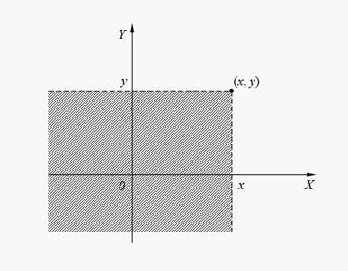
In terms of distribution laws is fairly also the following definition: two random variables X and Y are called independent if distribution law of each of them does not depend on accepted value of another.

Joint function of distribution of system of two random variables ( X , Y ) is called probability of joint performance of inequalities X < х and Y < у :

(34)

Event means product (i.e. joint performance) of events { X < х } and { Y < у }.

Geometrical interpretation of joint function of distribution F ( x , y ) is probability of hit of random point ( X , Y ) on plane inside of infinite quadrant with top in a point ( x , y ) (the shaded area on Fig. 8).

Fig. 8. Geometrical interpretation of joint function of distribution F ( x , y )

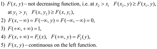
Basic properties of joint function of distribution:

(35)

Here

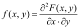
System of two random variables ( X , Y ) is called continuous system, if its joint function of distribution F ( x , y ) is continuous function differentiated on each argument and which has the second mixed private derivative . Both random variables X and Y – are continuous. Then function

(36)

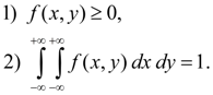
is called joint density function of system of two random variables ( X , Y ).

Basic properties of joint density function:

(37)

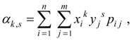
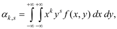
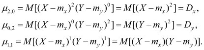
As numerical characteristics of system of two random variables X and Y initial and central moments of various orders are usually considered. Order of moment is sum of its indexes k + s .

Initial moment of the order k + s of system of two random variables X and Y is called mathematical expectation of product X ^k on Y ^s :

(38)

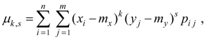
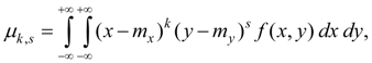
Central moment of the order k + s of system of two random variables X and Y is called mathematical expectation of product ( X – m _x ) ^k on ( Y – m _y ) ^s :

(39)

where m _x = М ( Х ), m _y = М ( Y ).

For system of discrete random variables X and Y :

(40)

(41)

where р _{i j} = Р { Х = x _i , Y = y _i }.

For system of continuous random variables X and Y :

(42)

(43)

where f ( x , y ) – joint density functionof system of random variables X and Y .

In engineering applications of mathematical statistics moments of the first and the second orders more often are used.

Initial moments of the first order

(44)

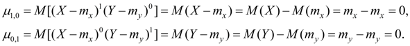
are mathematical expectations of random variables X and Y .

Central moments of the first order are always equal to zero:

(45)

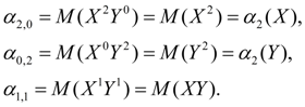
Initial moments of the second order

(46)

Central moments of the second order:

(47)

Here D _x , D _y – dispersions of random variables X and Y .

The central moment of the second order is called covariance of random variables X and Y .  Let's designate it :

.       (48)

From definition of covariance (48) follows:

(49)

The dispersion of random variable is in essence a special case of covariance:

(50)

From definition of covariance (48) we’ll receive:

(51)

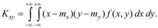
Covariance of two random variables X and Y characterizes a degree of their dependence and a measure of dispersion around of point . Often happens conveniently to express covariance in the form of:

(52)

Expression (52) follows from definition of covariance (48).

Dimension of covariance is equal to product of dimensions of random variables X and Y .

Dimensionless value describing only dependence of random variables X and Y , but not spreading:

(53)

is called coefficient of correlation of random variables X and Y .

This parameter characterizes a degree of linear dependence of random variables X and Y . For any two random variables X and Y coefficientof correlation . If , then linear dependence between X and Y increasing, if then linear dependence between X and Y decreasing, at linear dependence between X and Y is not present. At random variables X and Y are called correlated, at – not correlated. Absence of linear correlation does not mean absence of any other dependence between X and Y . If rigid linear dependence Y = aX + b , takes place, then at а > 0  and at а < 0.