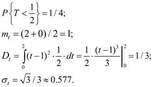
Examples [2]

E x a m p l e 1. Trains of underground go on a regular basis with an interval 2 minutes. Passenger leaves on platform during the casual moment of time which in any way has been not connected with the schedule. A random variable – time Т during which it should wait for a train. Find density function, mathematical expectation, dispersion, average square-law deviation and probability of what to wait to the passenger it is necessary no more half-minute.

S o l u t i o n . Density function f ( x ) =1/2 (0 < x < 2) is shown on Fig. 9.

Fig . 9. Density function

E x a m p l e  2. Random variable X has exponent distribution with parameter . Find probability of event {1 < X < 2}.

S o l u t i o n . We have The probability of hit in an interval (1, 2) is equal to an increment of function of distribution on this interval:

E x a m p l e  3. The matrix of distribution of system of two random variables X and Y is given by the table:

Find numerical characteristics of system of random variables ( X , Y ): mathematical expectations , dispersions , average square-law deviations , covariance and coefficient of correlation .

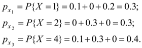
S o l u t i o n . First we’ll find series of distribution of separate values entering into the system. Summarizing probabilities p _ij , being in the 1-st, the 2-nd and the 3-rd lines, we’ll receive:

Series of distribution of random variable X looks like:

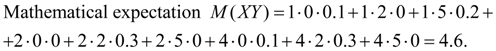
Mathematical expectation

From formula (8) dispersion

Average square-law deviation

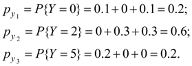
Similarly summarizing probabilities p _ij , being in the 1-st, the 2-nd and in the 3-rd columns, we’ll receive:

Series of distribution of random variable Y looks like:

Mathematical expectation

From formula (8) dispersion

Average square-law deviation

Covariance from formula (52) is equal to

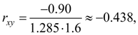Coefficient of correlation: thus, between random variables X and Y there is a negative linear correlation, i.e. at increase in one of them another has decreases.