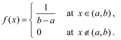
Distributions of continuous random variables

Uniform distribution. Continuous random variable X is distributed uniformly on interval ( a , b ) if all its possible values are on this interval and its density function is constant:

(29)

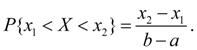
For random variable X uniformly distributed in interval ( a , b ) (Fig. 4), probability of hit in any interval ( x ₁ , x ₂ ), laying inside of interval ( a , b ), is equal to:

(30)

Fig. 4. Graph of uniform distribution density function

Examples of uniformly distributed values are mistakes of rounding up. So, if all tabular values of some function are approximated to the same digit then choosing at random tabular value, we consider, that mistake of rounding up of chosen number is a random variable uniformly distributed in interval

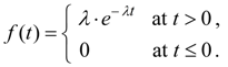
Exponent distribution. Continuous random variable X has an exponent distribution if its density function is expressed by the formula:

(31)

Graph of density function (31) is represented on Fig. 5.

Fig. 5. Graph of exponent distribution density function

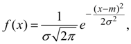
Time Т of non-failure operation of computer system is a random variable having exponent distribution with parameter λ , which physical sense – an average number of refusals in unit of time, not including idle times of system for repair.

Normal (Gaussian) distribution . Random variable X has normal (Gaussian) distribution if density function is defined by the dependence:

(32)

where m = M ( X ) , .

At normal distribution is called standard .

Graph of normal distribution density function (32) is represented on Fig. 6.

Fig. 6. Graph of normal distribution density function

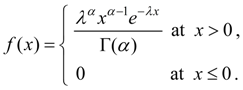
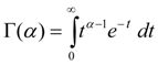
Normal distribution is the most often meeting in various casual natural phenomena. So, mistakes of performance of commands by automated device, mistakes of conclusion of spacecraft in the given point of space, mistakes of parameters of computer systems, etc. in the most cases have normal or close to normal distribution. Moreover, random variables formed by summing of great quantity of random addendum s, are distributed practically according to normal law.

Gamma distribution.

Random variable X has gamma distribution if its density function is expressed by the formula:

(33)

where – Euler’s gamma function.

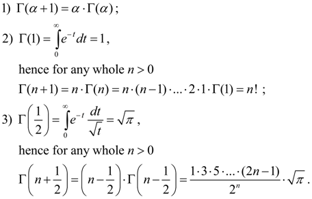
The basic properties of gamma function :

Parameters – any positive numbers. Gamma distribution is also Pearson’s distribution of type III [3]. At gamma distribution turns to exponent distribution with parameter λ , as Г (1) = 1. Gamma distribution is widely used in mathematical statistics. Graphs of gamma distribution density functions (33) at are presented on Fig. 7.

Fig. 7. Graphs of gamma distribution density functions