|
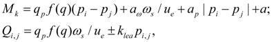
Library of hydraulic elements and their mathematical models The kind of the equations of base hydraulic elements depends, generally, on the assumptions accepted at decision of specific problems. As in this case we consider methods of computer-aided dynamic calculation, described by two basic features: automatic forming of mathematical model by a choice of necessary equations from the general library of mathematical models and construction on a basis of it programs of mass using oriented to application for hydraulic systems of arbitrary kind, it was necessary to choose from the big number of available models of elements the most common models, comprehensible to the decision as more as possible the broad audience of problems. Therefore for some hydraulic elements described with a various degree of detailed elaboration (pipeline, local resistance), the special researches [1] have been carried out by the author. The purpose of these researches was the comparative analysis of applied models for estimation of a degree of their adequacy at various external influences and parameters. As a result for mathematical description of hydraulic elements chosen as base ones the mathematical models reduced below have been accepted into which the following designations are entered: р – pressure; Q – flow; M – torque moment. Indexation of variables is made according to numbers of nodes in which the given variable (Fig. 1) operates. The library of equations of hydraulic elements reduced below basically can suppose their various mathematical descriptions under condition of preservation of the concept of a three-node element. Pump. For the pump description it is enough to write down the equation of moments on a shaft (node k ) and equations of flows in input (node i ) and output (node j ) in view of volumetric losses. Thus non-uniformity of the pump flow owing to kinematic features and compressibility of working fluid in sucking and pressure head cavities is not considered. In view of the accepted assumptions the pump mathematical model looks like [1, 2]:
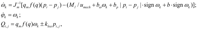
где q p – maximal geometric volume of pump; f (q) –parameter of regulation; – 1 ≤ f (q) ≤ 1; ω s – angular speed of diesel engine shaft; а ω , а р , а – coefficients of pump hydro mechanical losses depending on angular speed, pressure, and constant of hydro mechanical losses; u e – transfer number of gear between an engine and a pump; k lea – coefficient of pump volumetric losses (leakages); for Q i , p i the sign "plus" is accepted, for Q j , p j – the sign "minus". Values а ω , а р , а , k lea get out under the catalogue or from passport characteristics of mechanical and volumetric efficiency of the certain standard size pump. The hydro mechanical losses depending on pressure, are calculated on the module for an opportunity of consideration of brake modes and flow reversing (when f (q)< 0). Hydraulic motor. The mathematical model of hydraulic motor should to describe its dynamics (the equation of moments in node k , resolved relatively angular acceleration and written down in a normal form), and also the equations of flows in input (node i ) and output (node j ) in view of volumetric losses. Without taking into account non-uniformity of flow (it is similar to pump) the equations of the hydraulic motor look like [1, 2]:
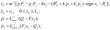
where ω k – angular speed of the hydraulic motor shaft; J m – moment of inertia of the hydraulic motor in view of rotating masses of working mechanism; q m – the hydraulic motor maximal geometric volume; f (q) – parameter of regulation; – 1 ≤ f (q) ≤ 1; М l – loading moment; b ω , b р , b – coefficients of hydraulic motor hydro mechanical losses depending on angular speed, pressure, and constant of hydro mechanical losses; u mech – transfer number of the working mechanism gear; k lea – coefficient of hydraulic motor volumetric losses (leakages); for Q i , p i the sign "plus" is accepted, for Q j , p j – the sign "minus". As well as for a pump, values b ω , b р , b , k lea choose under the catalogue or from passport characteristics of mechanical and volumetric efficiency of the certain standard size hydraulic motor. Hydro mechanical losses in the equation of the moments are written down in view of a shaft rotation direction (sign ω k ) and opportunities of consideration of a brake mode | p i – p j |. Hydraulic cylinder. Dynamics of hydraulic cylinder is described by the equations of progressive motion of piston (node k ) at action of pressure, external loading, forces of friction and the equations of flows on input (node i ) and output (node j ) in view of compressibility of fluid in cavities of the cylinder. On a basis of the standard assumption about absence of leakages in hydraulic cylinder with rubber and other soft seals the equations of the hydraulic cylinder dynamics look like [1, 2]:
where
v
k
– speed of the piston moving;
т
– mass of the hydraulic cylinder mobile parts reduced to a rod;
Coefficients of proportionality between pressures in cavities I (node i ) and II (node j ) and force of friction in cylinder seals:
k
and coefficients of elasticity of cavities with working fluid:
k
where
f –
coefficient of seal friction on the cylinder surface;
H –
height of seal;
Δ
V
E
=
here
Hereinafter a function of dry friction
f
(
v
k
) is written down for brevity in the form of
R
m
where P – moving force, a function of dry friction f ( v k ) will be defined as follows [2]:
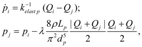
Such model of friction describes presence of stagnation zone at zero speed of a mobile part, for example, at starting. Pipeline. For description of dynamic processes in pipeline with a fluid the mathematical model with the concentrated parameters in input (node i ) and output (node j ) of pipeline, taking place at the following conditions is used: - wave processes are not considered; - losses of pressure on length depend on average value of flows in input and output; - inertial component of a working fluid is not considered. Then the mathematical model of pipeline with a fluid looks like [1, 2]:
где
k
here
d
E
=
где
here Re = 2 |
Q
i
+
Q
j
| / (
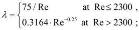
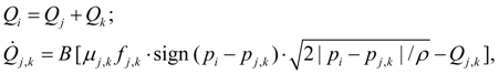
Deadlock site of pipeline (cavity). For a deadlock site of pipeline losses of pressure on length can be neglected, and then its equations of dynamics become:
where
here
d
E
=
where
Е
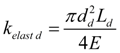
Local resistance (throttle). Flow of fluid through a throttle is connected with pressure difference in input (node i ) and output (node j ) by known dependence [1, 2]:
where
Use of flows equation (9) often is as the reason of instability of computing process because of aspiration to infinity of a derivative of a square root in zero (it takes place at small differences of pressures). The equation (9) defines the flow through a throttle in established mode of current of a fluid and, hence, does not consider inertial properties of fluid. More precisely dependence of flow through a throttle is expressed by the differential equation [3]:
where
l
– length of a fluid column in local resistance; besides for brevity of records here it is designated:
However the equation (10) is of little use for practical use. The matter is that the length
l
of a fluid column is defined not only constructive length of local resistance, but also length of a zone of unsteady current in output of throttle ("torch"), to define which even by experimental is very difficultly. Besides at consideration of adjustable throttle there are difficulties of computing character connected with discontinuity of the right part of the equation (10) at
which is deprived the specified lacks and asymptotic solution of which coincides with the solution of equation (9). Here
B
– the parameter considering inertia of a fluid column and depending on
l
and some other values (
The equations of flows for other kinds of local resistance (tees, valves, pilot operated check valves, directional control valves) are similar to the equations (11). Tee (divider or adder of flows). The equations of flows in tee nodes i , j , k at division of flow look like [1, 2]:
where
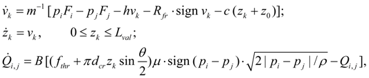
Valves. The direct action valve is described by equations of movement of locking-regulating element (node k ) and equations of flows (nodes i and j ) [1, 2]:
where
v
k
– speed of movement of
locking-regulating element
;
m
– mass of valve moving part;
F
i
and
F
j
– working areas of
locking-regulating element
from pressure head and drain lines;
h
– coefficient of viscous friction;
R
fr
– force of dry friction;
с
–rigidity of spring;
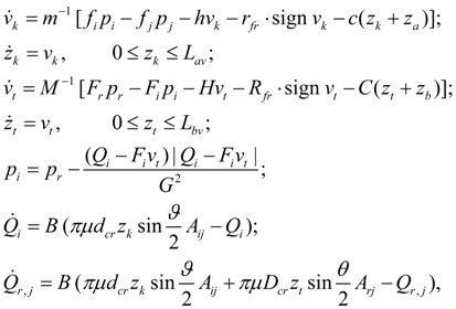
These equations concern to pressure relief and check valves. The corresponding equations for reducing valve have insignificant differences. In the equations (13) a hydro dynamical force which essential influences only on static characteristic of valve [2] is not considered. The indirect action valve can be presented in the form of two elements: a main valve with nodes r , s , t and a pilot valve with nodes i , j , k . If node j is general for both valves, i.e. s = j then mathematical model of the indirect action valve looks like [1, 2]:
where
v
k
,
z
k
– speed and displacement of
locking-regulating element
of pilot valve;
v
t
,
z
t
– speed and displacement of
locking-regulating element
of main valve;
т
and
М
– masses of moving parts of pilot and main valves;
Hydraulic accumulator. For the description of dynamics of hydro pneumatic or spring accumulator it is necessary to write down equations of piston (membrane) movement in node k , equation of pressure in input (node i ) and equation of polytropic process in a gas cavity (node j ) [1, 2]:
where
т
– mass of a mobile part of hydraulic accumulator;
F
=
k
here
Δ
V
E
=
here
Е
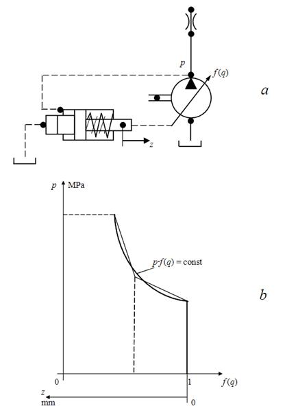
Power regulator
is intended
for
maintenance of constancy
of power selected
from engine
pQ
= const. Actually, power regulator provides a constancy of value:
p
·
f (q)
= const in the certain working range of pump. However, considering, that
Fig. 2. Static characteristic of power regulator
Then power regulator is described by the following system of equations [1, 2]:
where
т
– mass of mobile part of power regulator;
А
– coefficient considering for axial-piston pumps the additional moment, acting to swinging unit;
F
– working area of plunger under pressure of each of two pipelines;
Pilot operated check valve.
Pilot operated check valves are used for fixing and control of lowering of working bodies which are being under action of external loadings, in hydraulic systems of building machines (cranes, loaders, winches). On Fig. 3 simplified circuit of pilot operated check valve and diagram of its connection in hydraulic system is shown. At submission of fluid
1
in cavity under valve
3
it works as usual check valve, passing flow of working fluid to hydraulic cylinder. At submission of fluid
1
under piston of pusher
2
it compulsorily opens the valve, providing passage of flow through throttle from of hydraulic cylinder at piston lowering. On the scheme indexes
i
,
j
,
k
designate nodes accordingly of input, output and moving of valve, and by indexes
r
,
s
,
t
– nodes accordingly of input, output and moving of pusher.
Pilot operated check valves are issued in two modifications: with general drain of pusher and valve (in this case
r
=
i
) and with separate drain (then
r
Fig. 3. Pilot operated check valve and its connection in hydraulic system.
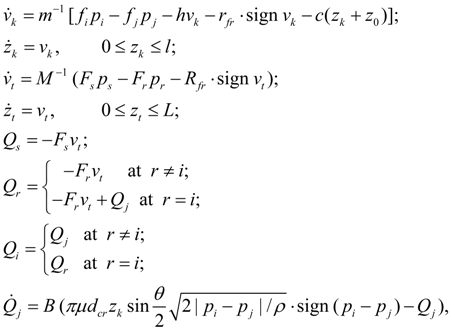
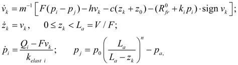
Depending on, whether there are pusher and valve in contact or not, dynamics of pilot operated check valve is described by two various mathematical models. In the time moment of contact occurrence when pusher starts to influence the valve, there is their impact that leads to necessity of correction of coordinates according to existing dependences of theory of shock systems. At absence of contact of pusher and valve dynamics of pilot operated check valve is described by the following system of equations [1, 2, 4]:
where
т
and
М
– masses of valve and pusher;
At approach of pusher and valve contact, when
and at absence of impact both bodies move in common, therefore their movement is described by the system of equations:
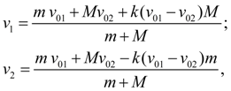
where х 0 – initial clearance between pusher and valve. The given model is incomplete as, considering great speeds and geometry of mobile parts which contact can be considered as the central impact of elastic cores, would be incorrect to consider, that at performance of conditions (18) the system instantly passes from condition described by the equations (17) in condition, described by the equations (19). It speaks about necessity of introduction of transitive shock mode model.
It is possible to apply formulas of classical hypothesis of impact to considered shock system "pusher-valve". Let before impact body in mass of
m
had speed
where
Preliminary computations of the accepted shock model at k = –0.5 have shown, that arising high-frequency shock fluctuations of valve concerning pusher have enough small amplitude, and besides, as a result of their attenuation there comes such moment when values of rebounds can be neglected, considering pusher and valve «agglutinate» [see equations (19)]. Therefore impact of pusher about valve as a result has been accepted not elastic (coefficient of restoration k = 0). After impact recalculation of pusher and valve speeds from formulas (20) is made at k = 0, i.e. speeds of both bodies are accepted equal to speed of their center of masses, and the further movement is considered as joint. Directional control valve. Directional control valve represents a complex of local resistances formed by its channels and connecting nodes adjoining them r and s . Flow through each such local resistance is expressed by equation similar to the equation (11):
where
In intermediate position of spool channels can be crossed in one node in which, hence, there will be a summation or division of flows of working fluid. Therefore flows in nodes belonging simultaneously various channels of directional control valve, turn out summation of flows through corresponding channels converging in given node. Hence,
where
i
, … ,
m
– numbers of directional control valve nodes;
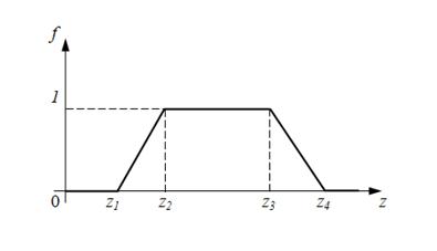
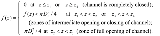
Change of through passage sections of channels of directional control valve can be approximated, for example, by trapezoidal characteristic, unequivocally defined by four positions of spool:
Fig. 4. Dependence of through passage section area of channel on spool displacement.
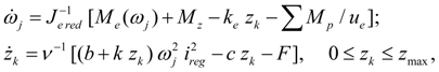
Diesel engine with a centrifugal regulator. Dynamics of diesel engine with a centrifugal regulator is described by equation of torque moments on the engine shaft (node j ) and equation of regulator muff movement (node k ) [1]:
where
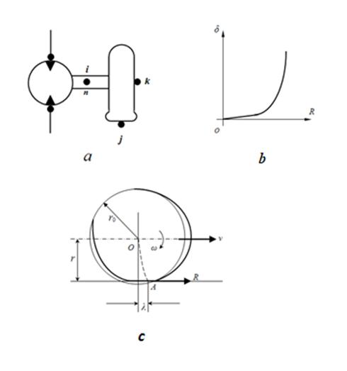
Wheel (wheel mover). For carrying out of tractive-dynamic calculations of hydraulic volumetric transmissions of self-propelled wheel machines it is necessary to consider wheel (wheel движитель ) as one of base elements – Fig. 1. Indexes i , j , k designate on the scheme accordingly nodes of input (power shaft of wheel), output (point of contact of wheel with road) and moving of machine. The considered here model of wheel mover describes rigid communication of wheel with the hydraulic motor, i.e. possible elastic deformations of gear and shaft between hydraulic motor and wheel are not considered.
Fig. 5. To conclusion of equations of dynamics of wheel. а – simplified diagram, b – slipping curve, в – deformation of tire.
In view of the accepted assumptions mathematical model of dynamics of a wheel (wheel mover), Fig. 5 а , looks like:
where
М
i
– wheel moment in view of losses in gear;
М
n
– moment reduced to shaft of hydraulic motor;
In established mode
wheel circular force
R
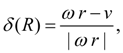
is connected with relative slipping
where
Here ω – wheel angular speed; v – speed of machine progressive movement (node k , Fig. 1).
Value of dynamic radius of wheel
r
depends on static deflection of wheel under loading
where
In unsteady mode
the dependence (26), having static character, should be replaced by dynamic model. For this purpose we’ll take advantage offered in [5] technique, according to which wheel circular force
R
is function of longitudinal deformation
In established mode
i.e. in established mode slipping function
Elements of control systems (typical linear dynamic parts of automatic control) . In control systems of volumetric hydraulic drive various physical devices are used: hydraulic, electromagnetic, electro hydraulic, etc. Therefore at solution of dynamics problems of hydraulic systems it is necessary to simulate various by nature systems of control and regulation. The majority of them is well described by means of typical linear dynamic parts of automatic control [7], to which the following links are related: 1) an ideal intensifying (no inertial) link – an adder; 2) the 1-st order aperiodic (inertial) link; 3) the 2-nd order aperiodic link; 4) an oscillatory link; 4a) a conservative link (a special case of an oscillatory link); 5) an ideal integrating link; 6) an inertial integrating link; 7) an ideal differentiating link; 8) an ideal link with introduction of derivative; 9) an inertial differentiating link; 10) the 2-nd order dynamic link (the general case). Mathematical models of the listed linear dynamic links are written in the form of ordinary differential equations, instead of in operational form (in the form of transfer functions) as transient processes are interested for us in time area, instead of in frequency area. Generally the 2-nd order linear dynamic link is described by the equation:
where
For all other types of dynamic links their equations are received as special cases (31): an ideal intensifying (no inertial) link – an adder:
the 1-st order aperiodic (inertial) link:
the 2-nd order (aperiodic or oscillatory) link:
a conservative link:
an ideal integrating link:
an inertial integrating link:
an ideal differentiating link:
an ideal link with introduction of derivative:
an inertial differentiating link:
Thus, all typical linear links can be incorporated in one generalized element LINK (the identifier of this element in library of base elements) with nodes i (input), j (output), k (an additional input for the link – adder). Considering specificity of hydraulic systems, in the right parts of equations of dynamic links as entrance signals pressures can be added:
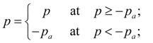
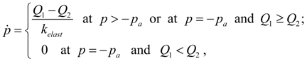
Conditions, restrictions, comments. It is necessary to add the resulted equations of linear dynamic links by some restrictions reflecting physical properties of variables, and also some design features of devices (for example, detents of mobile parts). As in the equations superfluous pressure is considered, performance of the conditions is necessary:
where
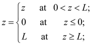
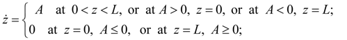
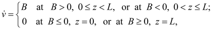
In some real elements movement z of mobile parts is limited by detents. Such nonlinearity can be written in the form of inequalities:
where
L
– maximal value of movement
z
;
А
– right part of the differential equation resolved respect to
Let's notice, that the equations for definition of pressure are included into the description of those elements which contain significant in comparison with other elements volumes of working fluid (for example, hydraulic cylinders, pipelines, including deadlock, hydraulic accumulators). Therefore these elements in simplified diagram should be divided by other hydraulic devices in which compressibility of fluid can be neglected and which equations serve for definition of flows (for example, hydraulic cylinder cavity and pipeline, hydraulic accumulator and pipeline, or two consistently connected pipelines, should be divided by throttle or local resistance that does not contradict physical sense). It allows to receive the closed system of equations for definition of pressure and flows in junctions of hydraulic elements. |
Contents
>> Engineering Mathematics
>> Hydraulic Systems
>> Dynamic Analysis
>> Library of hydraulic elements and mathematical models
 ,
,


 ,
,