|
Library of base elements and their mathematical models
The kind of base elements equations always depends on the assumptions accepted at the solution of the specific problems. As in the given case methods of
computer-aided
dynamic calculation are considered, described by two basic features: automatic forming of mathematical model by a choice of the necessary equations from the general library of mathematical models and construction on a basis of it general using programs applied to drives of arbitrary kind, it was necessary to choose from the big number of base elements models the most common available models, comprehensible to the solution as more as possible the broad field of problems. As a result for the description of base elements of mechanical and hydro mechanical transfers the resulted below mathematical models have been accepted in which following designations are used:
v
– linear speed;
The resulted below library of equations of typical elements basically can suppose their various mathematical description at condition of preservation of the concept of a three-node element.
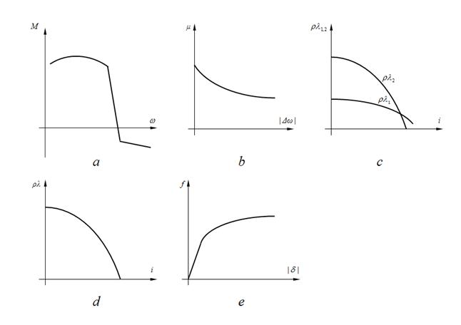
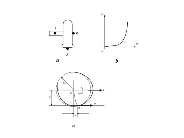
Characteristics of elements of mechanical and hydro mechanical drives resulted on Fig. 3, are approximated by a final set of points
Fig. 3. Characteristics of base elements of mechanical and hydro mechanical transfers: a – diesel; b – frictional clutch; c – hydraulic torque converter; d – hydro dynamic clutch; e – wheel (slipping curve).
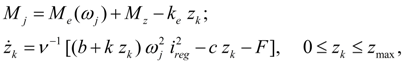
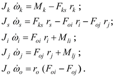
Diesel engine with a centrifugal regulator. The diesel engine with a centrifugal regulator is described by system of equations of the shaft moments (node j ) and the regulator muff movement (node k ) [1, 2]:
where
At simulation of transient processes often it is necessary to pass in area of partial (regulator) characteristics of a diesel engine that in real conditions is provided with change of
F
– force of preliminary compression of the spring adjustable by the driver by means of a control lever. Generally value of
F
varies from 0 up to a maximum
where
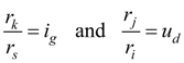
Gear. In a gear (Fig. 1) a constancy of transfer ratios in nodes i , j , k , takes place, i.e.
where
Let efficiencies of a gear in branches
where
Elastic shaft. A torque moment developed due to elastic angular deformation, depending also from damping properties of a shaft and enclosed in nose j (Fig. 1), is equal to:
where
c
– a shaft angular rigidity;
h
– coefficient of viscous friction;
The moment of an opposite sign operates in node
i
:
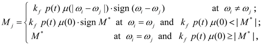
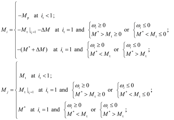
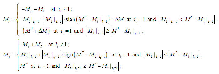
Frictional clutch. The moment developed by a frictional clutch and enclosed in node j (Fig. 1), is equal [1, 2] to:
where
The moment of an opposite sign operates in node
i
:
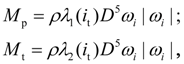
Hydraulic torque converter.
The moments developed on pump (
and besides
Here
D
- active diameter of work wheels of hydraulic torque converter,
Coefficient of transformation by definition is equal to:
Then
If hydraulic torque converter is executed structurally with overtaking clutch, then in blocking mode of pump (node i ) and turbine (node j ) wheels (in detail blocking mode see in the section «Blocking of frictional clutches and hydraulic torque converters» ) we’ll receive:
where
If pump and turbine wheels of hydraulic torque converter are blocked by a friction clutch, then in blocking mode pump (node i ) and turbine (node j ) wheels (in detail blocking mode see in the section «Blocking of frictional clutches and hydraulic torque converters» ) we’ll receive:
where
and at equality of angular speeds
Hydro Dynamical Clutch . A moment, realized by hydro dynamical clutch:
where
D
- active diameter of work wheels of hydraulic dynamical clutch,
As at
Wheel (wheel mover). For carrying out of tractive-dynamic calculations of hydro mechanical transmissions of self-propelled wheel machines it is necessary to consider as one of base elements a wheel (wheel mover) – Fig. 1. On the scheme indexes i , j , k designate accordingly nodes of an input i (a power shaft of a wheel), an output j (a point of contact of a wheel with road) and machine movement k .
Fig. 4. To a conclusion of equations of a wheel dynamics.
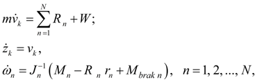
In view of the accepted assumptions mathematical model of a wheel (wheel mover) dynamics, Fig. 4, looks like [1, 2]:
where
т
– machine mass;
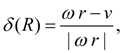
In the settled mode
a circle force
R
on a wheel is connected with relative slipping
where
Here ω – an angular speed of wheel; v – a speed of progressive machine moving (node k , Fig. 1).
The value of dynamic radius of wheel
r
depends on a static deflection of wheel under loading
where
In the
unsteady mode
dependence (25), having a static character, should be replaced by dynamic model. For this purpose we’ll take advantage offered in of [3] technique, according to which a circle force
R
on a wheel is a function of longitudinal deformation
In the settled mode
i.e. in the settled modea function of slipping
Thus, the mathematical model of a wheel (wheel mover) consists of the equations (24) and (28). Differential. The differential is one of elements dividing the drive scheme on sites for which nodes i and j of differential axes are either initial (at a branching of a power stream), or final (at summation of a power streams) – Fig. 5.
Fig. 5. The kinematic scheme of differential.
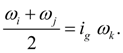
Angular speeds of differential axes are connected with an entrance shaft speed by following kinematic dependence:
whence
where
For symmetric differential
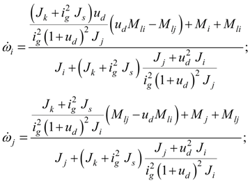
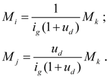
Torque moments in nodes i , j , k (Fig. 5) are connected by relations:
Then, knowing the moment
It means, that the node k cannot be carried to any site that is considered in algorithm of the structural analysis as a result of which nodes i and j are either initial (if in the scheme there are elements which first nodes coincide with nodes i and j of differential), or final (if in the scheme there are elements which second nodes coincide with nodes i and j of differential), and the node k is not included into one of sites and necessarily is a node of an elastic shaft . It does not limit a generality of the problem solution, but allows to receive rather easily values interesting us. Let's write down the equations of dynamics of differential axes in view of its geometry, kinematics and operating forces and moments (Fig. 5).
Input preconditions and the basic idea of a conclusion of these equations belong to Dr. L.B.Zaretsky. We’ll enter a number of additional designations:
Considering, that
Thus, the mathematical model of differential consists of the equations (31), (33) and (35). |
Contents
>> Engineering Mathematics
>> Hydro Mechanical Drives and Transmissions
>> Dynamic Analysis
>> Library of base elements and mathematical models
 (20)
(20)


 , and also including
