|
Control Systems - Dynamic Synthesis - Method of the movement law planning - Algorithm
Algorithm
Unlike
previous
this method allows synthesizing control without
use of frequency characteristics of drive. In most general case for planning the movement law (trajectory) it is necessary to solve two problems [1]:
1) a
problem of splitting
of control time interval [0,
Т
] on fineer pieces [
t
j
– 1
,
t
j
]
which boundary points
t
j
(nodes of interpolation) are defined often by a method of successive approximations;
2) a
problem of interpolation
– approximations of functions (operating signals)
y
(
t
) on an interval [0,
Т
]. One
of the most perfect ways of interpolation of functions is
the spline
interpolation
[1, 2].
In the problem statement considered by us about control of positioning of a cargo splitting of an interval [0,
Т
] on fineer pieces without
restriction a generality is not mandatory. Therefore in this case the problem reduces to planning of the law of movement of a cargo by a polynomial
of
n
-th degree which factors are defined, proceeding from the given boundary conditions.
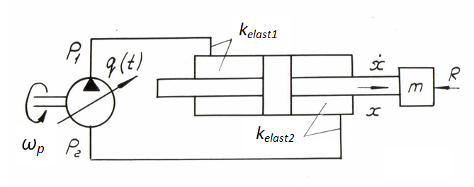
Fис. 1.
Let's consider again mathematical model of hydraulic system (Fig. 1), but now in view of leakages of working liquid, losses of pressure on length
of pipelines and in local resistances, having accepted the following assumptions:
1) losses of pressure depend on average value of working liquid flow on the pump output and on the hydraulic cylinder input;
2) reduced mass and load on the hydraulic cylinder rod, and also frequency of rotation of the pump shaft are constant;
3) parameters of working liquid (density, viscosity, module of volumetric elasticity) are constant;
4) dynamics of the control mechanism of the pump flow at the given stage is not considered.
As already it was marked above, its account does not represent basic difficulties, as this problem can be easily solved after or in parallel
considered, when required dependence of working volume of the pump
q
(
t
) (or even its current numerical value) is already known.
For this purpose it is necessary to write mathematical model of the control mechanism which output is
q
(
t
).
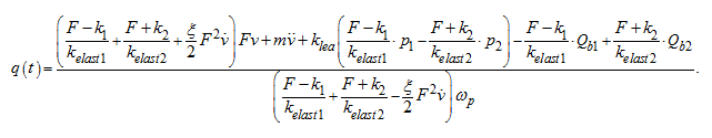
Then the system of equations of the hydraulic system (Fig. 1) dynamics becomes:
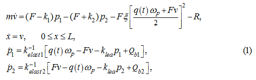
where
Q
b
1
,
Q
b
2
– boost flows in pipelines of the hydraulic system,
ξ
– the
reduced factor of hydraulic resistances; other designations the same, as earlier:
m
– mass of the mechanism mobile parts reduced to a rod;
р
1
,
р
2
– pressures in pressure head and drain cavities of the hydraulic system;
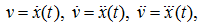
x
,
v
–
movement and speed of the hydraulic cylinder piston;
k
1
,
k
2
– factors of proportionality in variable
components of force of friction, depending on pressure;
R
– a constant load on the hydraulic cylinder rod;
ω
p
–
angular speed of the pump shaft;
F
– the working area of the hydraulic cylinder piston;
q
(
t
) – working volume of the
pump in function of time (actually a control signal);
k
elast
1
,
k
elast
2
– factors of
elasticity of thehydraulic system cavities.
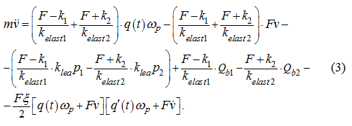
Differentiating the first of the equations (1) on
t
, we'll receive:

Substitution
 from the equations (1) in the equation (2) gives:
From the equation (3) in view of that

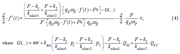
Let's notice, that
 whence, neglecting the left part of the expression (4), in view of infinitesimality of value
ξ
(
ξ
≈
1.6·10
-6
)
,
we'll finally receive:
whence, neglecting the left part of the expression (4), in view of infinitesimality of value
ξ
(
ξ
≈
1.6·10
-6
)
,
we'll finally receive:
 (5)
(5)
As calculations have shown
 therefore, if to neglect this summand, we'll receive simpler in comparison about (5) dependence
q
(
t
):
therefore, if to neglect this summand, we'll receive simpler in comparison about (5) dependence
q
(
t
):
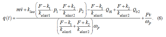
Running forward, we'll note, that calculations of transients in the hydraulic drive (Fig. 2) at variation of working volume of the pump
q
(
t
)
on the equations (5) and (6) made practically identical results.
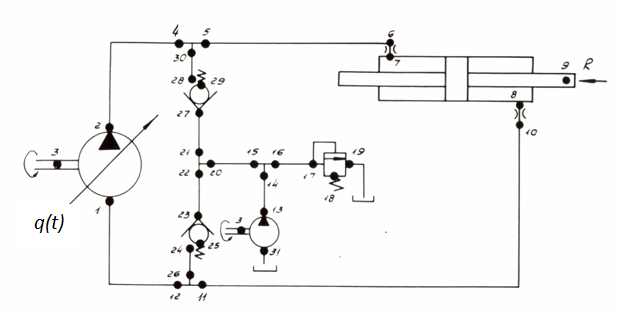
Fig. 2.
Having planned a trajectory
x
(
t
), we'll receive dependences
 which then it is necessary to substitute in the equations (5) or (6). As to pressure
р
1
and
р
2
, and also
boost flows
Q
b
1
and
Q
b
2
in pipelines of the hydraulic system their definition even
by means of simplified mathematical model (1) through
x
(
t
),
v
(
t
) and their derivatives is too complex in view
of existing essential nonlinearities and the high order of system of the equations, therefore during synthesis of the required law of control
q
(
t
) were substituted instead of
р
1
,
р
2
,
Q
b
1
and
Q
b
2
their numerical values received on each step of time as a result of modelling, that is carrying out analogy of
measurement of missing values. Such method provides among other things the partial compensation of the possible errors which are appearing owing to
the simplified mathematical description (1) of object of control. The result of influence of not considered factors in the certain degree is
reflected in "measured" sizes.
which then it is necessary to substitute in the equations (5) or (6). As to pressure
р
1
and
р
2
, and also
boost flows
Q
b
1
and
Q
b
2
in pipelines of the hydraulic system their definition even
by means of simplified mathematical model (1) through
x
(
t
),
v
(
t
) and their derivatives is too complex in view
of existing essential nonlinearities and the high order of system of the equations, therefore during synthesis of the required law of control
q
(
t
) were substituted instead of
р
1
,
р
2
,
Q
b
1
and
Q
b
2
their numerical values received on each step of time as a result of modelling, that is carrying out analogy of
measurement of missing values. Such method provides among other things the partial compensation of the possible errors which are appearing owing to
the simplified mathematical description (1) of object of control. The result of influence of not considered factors in the certain degree is
reflected in "measured" sizes.
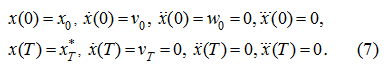
The law of movement
x
(
t
) we'll plan, proceeding from that during 0 ≤
t
≤
T
it is necessary to move a cargo from
a point
х
0
to a point
x
T
*
at the following boundary conditions:
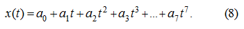
As shown from dependence (6) and system of the equations (1), an availability of
 is necessary for definition
q
(
t
). Having 8 boundary conditions (7), we'll plan the law of movement by means of a polynomial of
7-th degree:
is necessary for definition
q
(
t
). Having 8 boundary conditions (7), we'll plan the law of movement by means of a polynomial of
7-th degree:
From (7) – (8) we have:
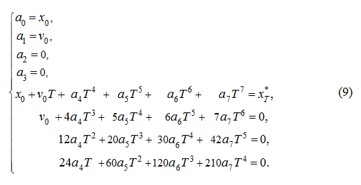
As the piston movement is considered from the left support (
х
0
= 0,
v
0
= 0) solving the system of equations
(9) rather
а
4
,
а
5
,
а
6
and
а
7
, we'll receive the following factors
of the polynomial:

For definition of control time
Т
it is necessary to consider a number of restrictions, first of which it is imposed on peak pressure
р
1max
:
р
1max
≤
р
1
*
, (11)
where
р
1
*
– the maximum allowable pressure in a pressure head cavity at dispersal (or in a drain cavity at braking),
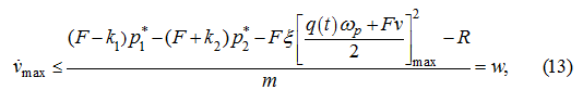
appropriating pressure of operation of a pressure relief valve. Differently, the restriction (11) is necessary that the maximal speed of system
was provided
without operation of a pressure relief valve
as differently the system becomes "badly operated" (there is affects influence of
the valve on transients), and speed of executive mechanisms decreases in view of pass-by of working liquid part through the valve.
At condition of sufficient working liquid boost pumping (
р
2
=
р
2
*
) from the first equation of the
system (1) and restrictions (11) we have the following approximate evaluation:
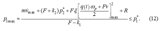
The expression (12) gives only approximate estimation for
р
1max
as speeds (flows) reach their maximal values later, than
acceleration, therefore actual value of peak pressure at the given parameters of regulation (
q
(
t
),
Т
and so forth) will
be a little below so, some stock on pressure
р
1
will be provided.
From (12) we'll receive:
and from (8) and (10) follows:
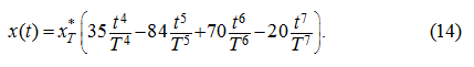
Differentiating (14) twice on
t
, we'll receive:
For a finding
 let’s differentiate (15) once again on
t
and equate
let’s differentiate (15) once again on
t
and equate
 to zero:
or after simplifications:
Having designated
 ,
we'll receive the following equation:
,
we'll receive the following equation:
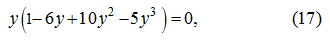
which roots are
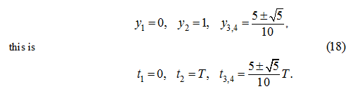
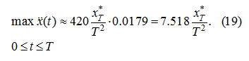
The analysis of roots (18) shows, that
 is reached at
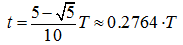 and it is equal:
From (13) and (19) follows:
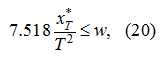
whence we'll finally receive an assessment "at the bottom" for time
Т
of transient:
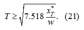
Having chosen
Т
from the condition (21), it is necessary to make check of restriction of current working volume of the pump (a control signal):
Direct definition
Т
from the condition (22) is interfaced to significant computing difficulties [see formulas (5) – (6)], therefore we'll
be limited to an assessment
q
(
t
), based on the following assumptions:
1) the maximum
q
(
t
) coincides on time with
v
max
;
2) variation of pressure in a drain pipeline at dispersal can be neglected, that is to accept, that

The first assumption is fair for enough smooth inclusions of the hydraulic system, and the second – at maintenance of boost flow necessary for the
compensation of leakages.
Let's address again to the system (1). Adding last two equations and considering, that
 as at dispersal
Q
b
1
= 0 we'll receive:
as at dispersal
Q
b
1
= 0 we'll receive:
Substitution (23) in (5) after simple algebraic transformations gives:
Substitution in (24) of expression for
 from the equation (1) after permit rather
q
(
t
) gives:
from the equation (1) after permit rather
q
(
t
) gives:
Let's notice, that at
 therefore according to (25) and the first accepted assumption we'll receive:
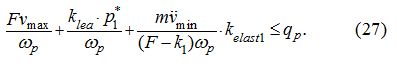
If the right part of the inequality (26) does not surpass
q
p
the inequality (22) takes place, therefore we'll consider a correlation:
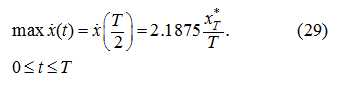
As follows from (14),
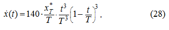
then apparently, that the maximum of speed
 is reached at
 and is equal:
Differentiating (28) twice on
t
, we'll receive the expression:
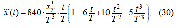
which minimum is reached at
and is equal:
Substituting (29) and (31) in (27) accordingly instead of
 ,
we'll finally receive:
,
we'll finally receive:
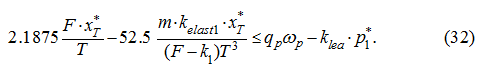
Thus, after choice
Т
from the condition (21) it is necessary to check up performance of the inequality (32). If the last is satisfied at
chosen value
Т
, on it synthesis of control by the method of the movement law planning comes to the end. Otherwise, it is necessary to
correct
Т
and again to make check of the condition (32). We'll note, that the algorithm of definition
Т
constructed here by
virtue of symmetry of the hydraulic system extends and on process of braking. An existing asymmetry of efforts (forces of friction) will go to
a stock on peak pressures at braking that proves to be true results of modeling of transients (see further).
|