|
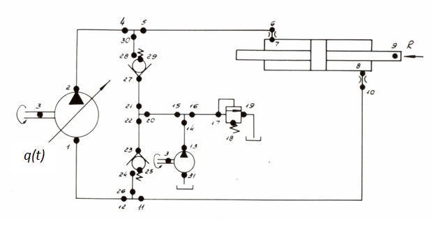
Example Let's address again to the rated hydraulic circuit diagram (Fig. 2) from the previous section "Algorithm" and consider on it the control algorithm stated above, modeling dynamics of a hydraulic drive by means of the program HYDRA.
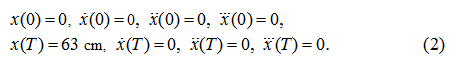
Fig. 2 Main parameters of the hydraulic system are given in tab. 1 of the previous section "Example" . Unlike the previous example, here it is adopted as final value of positioning of the hydraulic cylinder piston х Т * = 63 cm. Other parameters of the hydraulic system have been taken without changes.Let's plan the movement law
The value of losses of pressure on length of the pipeline and in local resistances is accepted here equal to 1.96 MPa (half of maximal value). In fact this value at the maximal acceleration as calculations have shown is a little bit less (1.5...1.96 MPa), that gives some stock on pressure р 1 . So, during dispersal (braking) it is necessary to implement of the condition: From the inequality (21) of the previous section "Algorithm" we have: In view of fulfillment of the condition (32) of previous section "Algorithm" it is accepted Т = 3 s. Then coefficients of the polynomial (1) describing the movement law, are equal:
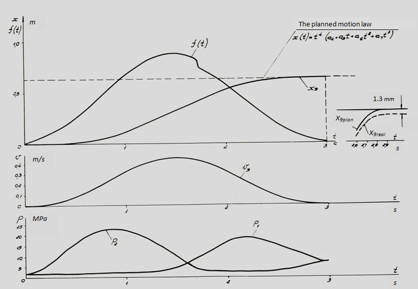
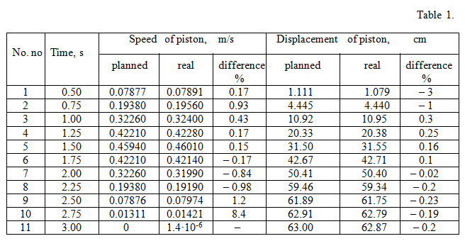
Fig. 3 Here, as well as earlier, are designated: р 1 , р 2 – pressures on an input and on an output of the basic pump (nodes 1 and 2), v 9 , х 9 – speed and movement of the hydraulic cylinder piston (node 9); f ( t ) – parameter of regulation of the pump flow, equal toFrom graphs of transients presented on Fig. 1 is visible, that as a result of control of the hydraulic drive according to the method of the movement law planning peak pressures do not exceed the given level ~25 MPa. Actual and planned movement laws have the insignificant differences shown in tab. 1.
The reason for these differences is distinction in the mathematical models of a hydraulic drive accepted in the program HYDRA and in the control algorithm (more simplified version), and first of all because of dynamics of boost system (for example, at t ≈1.72 s, apparently on Fig. 3, there is a jump of f ( t ) because of drastic change of boost flow at pressure р 2 drop), as well as of some nonlinear and inertial effects. The received maximal differences on the piston movement make 1.3 mm (see tab. 1). It is easy to see, that the received results confirm the basic assumptions accepted by development of the control algorithm, especially in that its part where the assessment of a maximum q ( t ) is made. So, the maximal values q ( t ) and v [on Fig. 3 – f ( t ) and v 9 ] almost coincide on time (the mismatch makes nearby 0.025 s); pressure in a drain pipeline р 1 does not change almost at t ≤ 1.4...1.5 s. Reached accuracy of positioning of the same order, when using the method of multiple periods of natural fluctuations. For reception of higher accuracy it is necessary, as it was already marked, introduction at a stage of "precise" control of special correcting links with feedback on movement, speed and probably on acceleration (pressure). However, these questions are beyond the given statement of the problem. |
Contents
>> Engineering Mathematics
>> Control Systems
>> Dynamic Synthesis of Control System of Hydraulic Drive
>> Synthesis of control by a power hydraulic drive of volumetric regulation
>> Method of the movement law planning
>> Example