Elementary transformations of matrices

Elementary transformations of a matrix find a wide application in various mathematical problems. For example, they lay in a basis of the known Gauss’ method (method of exception of unknown values) for solution of system of linear equations [1].

Elementary transformations of a matrix are:
1) rearrangement of two rows (columns);
2) multiplication of all row (column) elements of a matrix to some number, not equal to zero;
3) addition of two rows (columns) of the matrix multiplied by the same number, not equal to zero.

Two matrices are called equivalent if one of them is maybe received from another after final number of elementary transformations. Generally equivalent matrices are not equal, but have the same rank.

Calculation of determinants by means of elementary transformations

By means of elementary transformations it is easy to calculate a determinant of a matrix.

For example, it is required to calculate a determinant of the matrix:

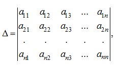
where .

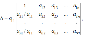
Then it is possible to bear a multiplier :

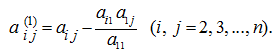
now, subtracting from elements of the j -th column appropriating elements of the first column, multiplied on , we’ll receive the determinant:

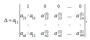
which is equal to where

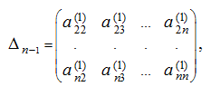
and

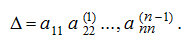
Then we repeat the same actions for and, if all elements 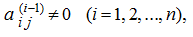then we’ll receive finally:

If for any intermediate determinant its left upper 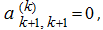element it is necessary to rearrange rows or columns in so that a new left upper element will not be equal to zero. If Δ ≠ 0 it always can be made. Thus it is necessary to consider, that the sign on a determinant changes depending on what element is the main one (that is when the matrix is transformed so, that ). Then the sign on an appropriating determinant is equal to .

E x a m p l e .  By means of elementary transformations result the matrix

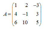
to a triangle type.

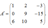
S o l u t i o n . First we’ll multiply the first row of the matrix by 4, and the second – by (–1) and add the first row to the second:

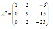
Now we’ll multiply the first row by 6, and the third – by (–1) and add the first row to the third:

Finally, we’ll multiply the second row by 2, and the third – by (–9) and add the second row to the third:

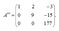
As a result the upper triangular matrix is received.