|
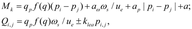
Library of hydraulic elements and their mathematical models Static calculation is a basic stage at designing hydraulic drives and transmissions of various machines and mechanisms. On a basis of results of static calculation synthesis of hydraulic circuit and selection of elements of the certain standard size is carried out. But at the same time it is closely connected with dynamic analysis as preliminary stage necessary for the correct giving of an initial condition of hydraulic system at simulating of transient processes. In resulted below equations of statics of hydraulic elements the same designations are accepted, and for the description of the input data of elements the same identifiers and tables are used, as at the dynamic analysis. Pump. For the pump description it is enough to write down equation of a shaft moments (node k ) and equations of flows in input (node i ) and output (node j ) in view of volumetric losses. Thus non-uniformity of the pump flow owing to kinematic features and compressibility of liquid in sucking and pressure cavities is not considered. In view of the accepted assumptions the mathematical model of the pump looks like [1, 2]:
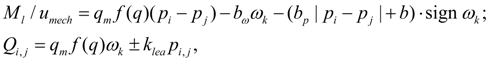
where q p – maximal geometric volume of pump; f (q) – parameter of pump geometric volume regulation; – 1 ≤ f (q) ≤ 1; ω s – angular speed of engine (diesel engine) shaft; а ω , а р , а – coefficients of pump hydro mechanical losses depending on angular speed, pressure, and constant value of hydro mechanical losses; u e – transfer number of gear between engine and pump; k lea – coefficient of pump volumetric losses; for Q i , p i the sign "plus" is accepted, for Q j , p j – "minus". Values of а ω , а р , а , k lea are chosen from the catalogue or from passport characteristics of mechanical and volumetric efficiency of the certain standard size pump. The hydro mechanical losses depending on pressure are calculated modulo for opportunity of consideration of brake modes and reversing flow (when f (q)< 0). Hydraulic motor. The mathematical model of hydraulic motor contains equation of moments in node k , and also equations of flows in input (node i ) and output (node j ) in view of volumetric losses. Without taking into account non-uniformity of flow (it is similar to pump) the system of equations of hydraulic motor looks like [1, 2]:
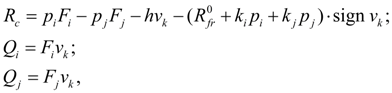
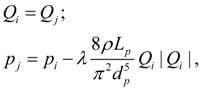
where ω k – angular speed of hydraulic motor shaft; q м – maximal geometric volume of hydraulic motor ; f (q) – parameter of hydraulic motor geometric volume regulation; – 1 ≤ f (q) ≤ 1; М l – loading moment; b ω , b р , b – coefficients of hydraulic motor hydro mechanical losses depending on angular speed, pressure, and constant value of hydro mechanical losses; u mech – transfer number of the working mechanism gear; k lea – coefficient of volumetric losses of hydraulic motor; for Q i , p i the sign "plus" is accepted, for Q j , p j – "minus". As well as for pump, values b ω , b р , b , k lea are chosen from the catalogue or from passport characteristics of mechanical and volumetric efficiency of the certain standard size hydraulic motor. Hydro mechanical losses in the equation of moments are written down in view of direction of shaft rotation (sign ω k ) and opportunities of consideration of a brake mode | p i – p j |. Hydraulic cylinder. Hydraulic cylinder is described by equation of balance of forces (forces of pressure, external loading, forces of friction) at piston progressive motion (node k ) and equations of flows in input (node i ) and output (node j ). On a basis of standard assumption about absence of leakages in hydraulic cylinder with rubber and other soft seals equations of statics of hydraulic cylinder look like [1, 2]:
where
v
k
– speed of piston motion;
F
i
=
π
(
D
k
Here f – coefficient of friction of seal material and cylinder wall; Н – height of seal. Pipeline. Mathematical model of pipeline with liquid consists of equality of flows in input (node i ) and output (node j ) and equations of losses of pressure on length and looks like [1, 2]:
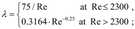
where
here Re = 4 |
Q
i
| / (
Deadlock site of pipeline (cavity). For deadlock site of pipeline losses of pressure on length can be neglected, and then equations of statics of deadlock site of pipeline become:
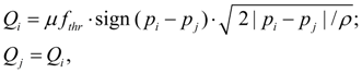
Local resistance (throttle). Flow of liquid through throttle is connected with pressure difference in input (node i ) and output (node j ) by the known dependence [1, 2]:
where
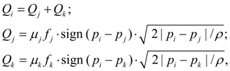
Tee (a divider or the summer of flows). Equations of tee flows in nodes i , j , k at division of flow look like [1, 2]:
where
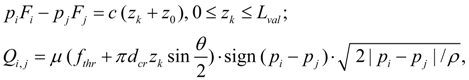
Equations of tee flows at summation of flows are similar (10), but have other values of flow coefficients. The assumption is accepted, that coefficients of hydraulic resistances at change of flow direction do not vary. Valves. Valve of direct action is described by equations of statics of locking-regulating element (node k ) and flows in nodes i and j [1, 2]:
where
F
i
and
F
j
– working areas of the valve
locking-regulating element
from pressure head and drain line;
с
– rigidity of spring;
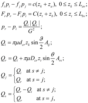
The resulted equations concern to pressure relief and check valves. The corresponding equations for reducing valve have insignificant differences. In equations (11) hydro dynamical force is not considered. Pilot controlled valve (of indirect action) consists of two elements: the main valve with nodes r , s , t and the pilot valve with nodes i , j , k . If a discharge node j is general for both valves, then s = j . Mathematical model of statics of pilot controlled valve looks like [2]:
where
Hydraulic accumulator. For the description of stationary mode of the hydro pneumatic or spring accumulator it is necessary to write down equations of balance of its piston (membrane) in node k , equation of flow in input (node i ) and equation of polytropic process in gas cavity (node j ) [1, 2]:
where
F
=
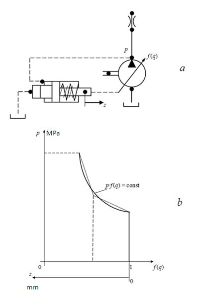
Power regulator
is intended for maintenance in the pump certain working range of constancy of the power taken away engine:
pQ
= const. Actually, power regulator provides a constancy:
p f
(
q
) = const. But,
Q = q
p
f
(
q
)
Fig. 2. Static characteristic of power regulator
Then in statics power regulator is described by the following equation [1, 2]:
where
А
– coefficient considering for axial-piston pumps the additional moment, acting to swinging unit;
F
– working area of plunger under pressure of each of two pipelines;
Diesel engine with a centrifugal regulator. Diesel engine with a centrifugal regulator in statics can be described by equation of engine shaft moments (node j ) and equation of regulator muff balance (node k ) [1, 2]:
where
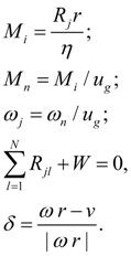
Wheel (wheel mover). For carrying out of traction calculations of hydro volumetric transmissions of self-propelled wheel machines it is necessary to consider as one of base elements a wheel (wheel mover) – Fig. 1. Indexes i , j , k designate accordingly nodes in input (power shaft of wheel), output (point of contact of wheel with road) and machine movement. The model of wheel mover considered here describes rigid communication of wheel with the hydraulic motor. In view of the accepted assumptions the static mathematical model of wheel (wheel mover) looks like:
where
М
i
– wheel moment in view of losses in gear;
М
n
– moment reduced to shaft of hydraulic motor;
In established mode
circular force
R
of wheel is connected with relative slipping
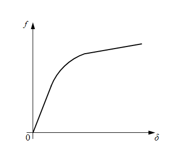
where
Fig. 3. Function of wheel slipping.
Here
f
(|
δ
|) – function of wheel slipping (Fig. 3);
ω
– angular speed of wheel;
v
– speed of machine progressive movement (node
k
, Fig. 1). Value of wheel radius
r
depends on static deflection of wheel
where
|
Contents
>> Engineering Mathematics
>> Hydraulic Systems
>> Static Analysis
>> Library of hydraulic elements and mathematical models