|
General scheme of solution The resulted above equations of statics of separate hydraulic elements contain some essential nonlinearity because of which solving of corresponding system of equations in final form (analytically) is impossible. Therefore for static calculation the iterative scheme of solution is used in which basis Newton-Raphson method lays. For application of this method it is necessary: - linearization of hydraulic elements equations; - the circuit structure analysis and minimization of number of unknowns; - giving of zero approach; - forming of matrix of coefficients of linearized equations with variable coefficients (owing to linearization in neighborhood of zero approach); - solving on each iteration of system linearized equations with variable coefficients. Linearization of equations of hydraulic elements it is executed at stage of construction of algorithm of static calculation. Zero approach is given by preparation of problem for solution together with input data. Other items of general scheme of solution are realized by program. Linearization of equations. Let the system of nonlinear equations is given: F l ( x 1 ,…, x N ) = 0, l = 1, … , N , (21) where x 1 ,…, x N – unknowns entering into these equations, F l – nonlinear functions.
Decomposing
F
l
(
x
1
,…,
x
N
) in power series in
neighborhood
of zero approach
F
l
(
l = 1, … , N . (22) Linearization of equations is a necessary preparatory stage as a result of which the algorithm and the program of static calculation of hydraulic systems are under construction.
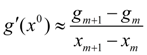
For realization of iterative process all graphic characteristics
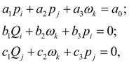
As to nonlinearities of kind | p i – p j | , sign ω k , sign v k in the equations of pump, hydraulic motor, e hydraulic cylinder and of some other elements, on each n -th iteration these functions can be considered as known values if to substitute instead of p i , p j , ω k , v k their values received on the previous ( n –1)-th iteration. Structural analysis of circuit and minimization of number of unknown persons. In each node of hydraulic circuit the following combinations of variables are possible: - pressure, liquid flow; - force, linear speed, linear movement; - torque moment, angular speed, turn angle. It allows to pass to integrated system of variables: "forces" (forces, pressures, torques), "speeds" (linear or angular, liquid flow), "movements" (linear or angular) which are indexed by numbers of circuit nodes. After linearization and transition to integrated system of unknowns it is possible to write down the equations of elements in a general view:
where
However, apparently from the equations (2) – (20) for static calculation, the number of unknowns can be reduced, as flows in input (node
i
) and output (node
j
) for a lot of hydraulic elements (for example, pipeline, throttle, valve) are equal. Therefore before forming of matrix of coefficients of system of linearized equations of hydraulic elements it is expedient to execute the structure analysis of the circuit for minimization of number of unknowns. It allows reducing considerably time of computer calculations, as number of operations which is carried out during solution of the
n
-th order system of linear algebraic equations is proportional to
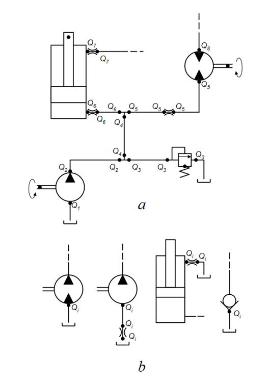
In any circuit of hydraulic drive there are sites within the limits of which in stationary mode flow of liquid does not vary. As it was already marked, these sites consist of pipelines, throttles, valves. At the same time the quantity of unknown flows in the circuit is defined by those hydraulic elements at which flows in input and output are various (pump, hydraulic motor, hydraulic cylinder, tee). The hydraulic circuit can be broken by these elements into sites along which the flow is constant, hence, each such site begins and comes to an end with one of the listed elements. Means, for numbering flows along the specified sites it is enough to number of them in output of the elements: pump, hydraulic motor, hydraulic cylinder, tee. As example on Fig. 4 а the arbitrary hydraulic circuit with numbering flows in nodes is presented from which it is visible, that actually number of unknown flows is equal to 8 while the general number of nodes in which it is required to define these flows, is equal to 18. We’ll note, that flows in all sites of the circuit, except for in what liquid acts from a tank thus will be numbered. Therefore, besides flows in output of the specified elements it is necessary to number also and flows in input lines of some elements connected to a tank (Fig. 4 b ).
Fig. 4. Numbering of flows a – in the circuit nodes, b – in input pipelines of hydraulic elements The algorithm of numbering of variables is reduced to the following. First the set of elements of the circuit "is looked through". Then according to the plant identification of base hydraulic elements the type of element depending on which flows and speeds are numbered is analyzed: 1) for pump the flow (its submission) in output (in node j ) receive the serial number; if the input of pump (node i ) is connected to a tank the serial number is appropriated also to the flow in input; 2) for hydraulic motor and hydraulic cylinder the flow in node j and speed in node k receive serial numbers; if node i is connected to a tank then flow in node i also receives serial number; 3) for tee : at division flows in node j and k receive serial numbers; at summation only flow in node k receives serial number; 4) for throttle and valve flow in node i if it is connected to a tank receives serial number; 5) for diesel engine angular speed in node j receive serial number. After this number of flow in input of each site is appropriated to flows in other nodes of the given site. After numbering flows and speeds unknown "forces" and "movements" are numbered therefore the new system of unknowns is received in which the first number "speeds" turns out, then – "forces" and at last – "movements". As shows the analysis, dimension of new system of unknowns on the average on 30 – 40 % are less, that leads to reduction of problem solving time in 3 – 4 times.
As a result of the circuit structure analysis to each node
M
the three of numbers
The stated algorithm of numbering of unknowns and minimization of their quantity is realized in the special program module of structure analysis of circuit and made automatically for everyone considered hydraulic circuit.
Formiong of matrix of coefficients.
The matrix of coefficients of system of linearized equations (22) is formed as follows. The identifier of any element defines group from
L
equations (24) of given element – submatrix coefficients of which form
L
lines of formed matrix. To numbers of nodes of element unequivocally there correspond numbers of new unknowns
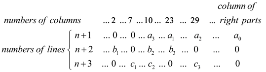
As illustration of process of matrix forming we’ll consider an example. Let the next element is the hydraulic motor with numbers of nodes i , j , k and let to the given time moment n lines of a matrix ( n equations) has been generated. We’ll write down linearized equations of hydraulic motor in a general view:
which get out according to the element identifier. We’ll assume, that as a result of structure analysis of circuit the unknowns entering into system of equations (25) have received the following numbers:
Other elements of matrix line [except for coefficients of equations (25)] are equal to zero. Then the following element gets out, etc. Process of matrix forming proceeds until elements of circuit are chosen all. Algorithm of solution of system of equations. For static calculation the iterative scheme of the decision is used in which basis the Newton-Raphson method lays. The system of linearized equations (22) in matrix form can be reduced to a kind: A [ x 0 ] x = B [ x 0 ], (26)
where
A
[
x
0
],
B
[
x
0
] – accordingly matrix of coefficients
On the n -th iteration the system of equations (26) becomes: A [ x n -1 ] x n = B [ x n -1 ], (27) where x n -1 – solution received on the previous ( n –1)-th iteration. Thus, on the n -th iteration from values x n -1 matrices A [ x n -1 ] and B [ x n -1 ] are calculated, and then the system of linear equations (27) is solved, therefore x n is defined. Process repeats until the given accuracy ε on everyone l –th component of vector x n will be satisfied:
Convergence of iterative process appreciably depends on a choice of consistent zero approach. We’ll notice, that often happens expedient for reception of correct zero approach to start a trial dynamic calculation of the same circuit with arbitrary initial conditions and with the external influences corresponding the considered stationary mode. Such transient process quickly enough converges asymptotically to the solution close to required zero approach and therefore, it can be accepted as demanded zero approach. |
Contents
>> Engineering Mathematics
>> Hydraulic Systems
>> Static Analysis
>> General scheme of solution