Examples

E x a m p l e  1. Solve the cubic equation with relative accuracy = 0.001 by Newton-Raphson method of tangents.

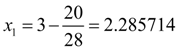
S o l u t i o n . In this case Hence, As zero approach we’ll accept = 3 (exact value of a root =2). Then from the formula (7) we’ll receive:

,

,

Let's check up, whether the given relative accuracy is reached:

.

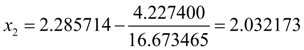
Let's continue iterations:

.

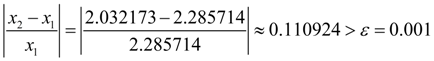
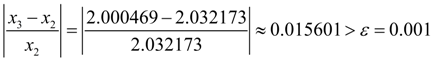
Again we’ll check up, whether the given relative accuracy is reached:

.

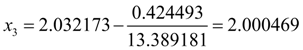
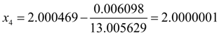
Following iteration to within six decimal signs gives practically exact value of a root:

.

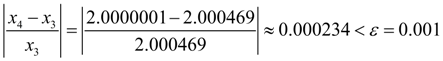
However, here again it is necessary to check up, whether the given relative accuracy is reached:

.

The found root of the equation is equal to 2.0000001. Thus, computing process has converged for 4 iterations, and we have received a required root with the given relative accuracy .

E x a m p l e  2. Solve the cubic equation with relative accuracy = 0.001 by the method of iterations.

S o l u t i o n . Let's copy the given equation in the form of (3):

where Then from the formula (4) we’ll receive:

The condition of convergence in this case looks like: but in this interval there are no roots of the equation . Moreover, for the function in a neighborhood of the root =2 the inequality takes place, that is the condition of convergence is not carried out and to search for the solution of the equation in the form of it is not meaningful, as numerical process will be divergent. Therefore it is necessary to write down the given equation in another way:

then and it is obvious, that in a neighborhood of the root =2 the inequality takes place, hence, the condition of convergence is satisfied. Therefore for the solution of the given cubic equation we’ll search from the formula:

Let's accept again as zero approach =3. Then we ’ ll receive :

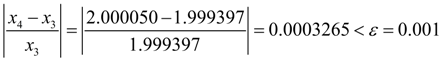
On this step the given relative accuracy is reached:

,

therefore process of a finding of a root of the equation can be considered completed. The found root of the equation is equal to 2.000050. Thus, here again the required root is found for 4 iterations with the given relative accuracy .

E x a m p l e  3. Solve the cubic equation with relative accuracy = 0.001 by the method of chords.

S o l u t i o n . Here Let's search for the solution on the segment [0, 4] (let's remind, that exact value of the root =2). Let's accept as zero approach =0. Then from the formula (12) we’ll receive:

On this step the given relative accuracy is reached:

,

and thus, process of a finding of a root can be considered completed. The found root of the equation is equal to 1.9986328. Here the required root is found for 12 iterations with the given relative accuracy .

E x a m p l e 4. Solve the cubic equation with relative accuracy = 0.001 by the method of halving.

S o l u t i o n . Here As initial we’ll consider the segment [0, 3], as on its ends the function F ( x ) accepts different signs: Then according to a condition of convergence (11) in the given example we’ll receive:

,

whence follows that is for achievement of the given accuracy of the solution of this equation by a method of halving into the segment [0, 3] it is required not less than 12 iterations.

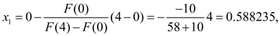
The sequence of actions in the method of halving is reduced to the following: on each step the next segment is considered, we halve it and we calculate value of function F ( x ) in the middle of this segment. Then we choose that half of segment on which ends the function F ( x ) has different signs. Results of the lead consecutive actions from the method of halving are tabulated:

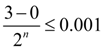
On 12-th step according to an estimation (11) the given accuracy of the solution is reached: ,

hence, for the solution of this equation with the given accuracy by the method halving into the segment [0, 3] it was required, predictably, 12 iterations. The found root of the equation is equal to 1.999878.

Let's notice, that if in the given example we have considered the segment [0, 4] as initial, that already on the first iteration we would receive the exact decision of the equation, as