|
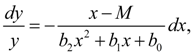
Alignment of statistical distributions. Pearson’s curves For alignment (approximation) of statistical distributions the set of various methods is used: polynomial approximation, Charlie’s series, Kramer's perturbation polynomials, Pearson’s method etc. The basic lack of polynomial approximation is formality of received distributions – the type of approximation is not connected with the nature of the random phenomenon. Charlie’s and Kramer’s methods are suitable to approximation of the distributions approached to normal. Unlike them Pearson’s method is universal enough and covers practically all known kinds of statistical distributions. Pearson [1, 2] has suggested to use for the description of statistical distribution of random variable X solutions of the differential equation:
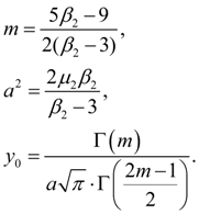
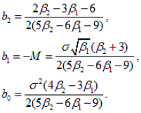
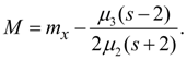
where as origin of counting х its average value serves, М – mode. Coefficients in the equation (1) can be calculated by means of the central moments .
At introduction of designations
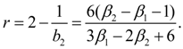
Let's enter auxiliary value:
Then the system of equations (2) can be written in the form of:
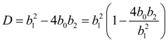
Let's calculate a discriminant of denominator in the equation (1):
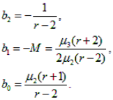
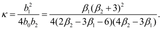
Let's designate
Then
The general integral of the equation (1) essentially depends on a kind of roots of a quadratic equation
1. At
2. At
3. At
To each of these cases there corresponds one of the basic types of Pearson’s curves – I, IV and VI. Other nine types and normal distribution curve – their private or boundary cases. Most often in an expert there are first seven types of Pearson’s curves. On Fig. 1 the graph for definition of type of a curve on parameters
Fig. 1. The graph for definition of Pearson’s curve type depending on
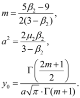
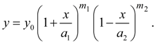
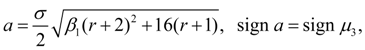
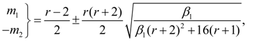
Let's consider the equations of Pearson’s curves of I – VII types and ways of definition of parameters entering into them [1, 2]. The curve of I type corresponds κ < 0; its equation looks like:
Exponents
and at
Coefficients
where
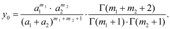
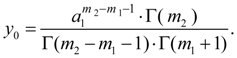
Initial ordinate
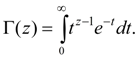
Here Г (z) – gamma-function :
Domain of curve
of
I
type is the interval:
Fig. 2. Pearson’s curves of I type
Depending on values
1. At
2. In case of different signs
3. At
The
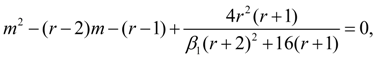
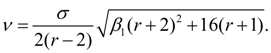
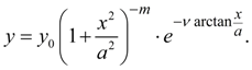
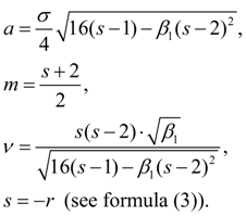
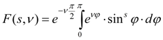
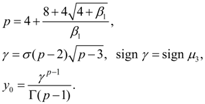
curve of IV type
corresponds
where
The sign of
ν
gets out opposite to a sign of
а
nd
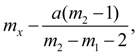
Origin of coordinates undertakes in a point
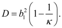
Fig. 3. Pearson’s curve of IV type The curve of VI type corresponds κ > 1 and is described by the equation:
Here
And the condition
Origin of coordinates undertakes in a point
The curve lies on an interval from
а
up to +∞ at
Fig. 4. Pearson’s curves of VI type
The following group of Pearson’s curves corresponds to private values of criterion κ .
The
curve of III type
takes place at
and
х
varies from –
а
up to +∞. The form of a curve – the same, as on Fig. 4 for the curve of
VI
type with replacement
т
1
on
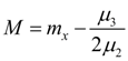
Mode
Special case of Pearson’s curve of
III
type at
Origin of coordinates – in a point
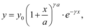
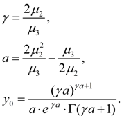
Curve of V type corresponds κ = 1. Its equation looks like:
Here
Function
y
=
f
(
x
) exists at all
х
> 0. Origin of coordinates – in a point
Fig. 5. Pearson’s curve of V type
At
κ
= 0 depending on value
The
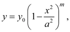
curve of II type
turns out at
where
Coefficient
The
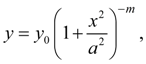
curve of VII type
corresponds
where
Coefficient
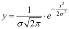
The curve of VII type is symmetric relatively origin of coordinates. The curve of normal distribution
turns out at
|
Contents
>> Applied Mathematics
>> Mathematical Statistics
>> Treatment of Experiment Results
>> Alignment of statistical distributions. Pearson’s curves

 – tabulated function.
 (here
(here
 and initial ordinate
 exists at

 General view of the curve is presented on Fig. 5.