The spline interpolation

Lagrange’s, Newton’s and Stirling’s interpolation formulas and others at use of big number of nodes of interpolation on all segment [ a , b ] often lead to bad approach because of accumulation of errors during calculations [2]. Besides because of divergence of interpolation process increasing of number of nodes not necessarily leads to increase of accuracy. For decreasing in errors all segment [ a , b ] is broken into partial segments and on each of them function is replaced approximately with polynomial of low degree. It refers to piece-polynomial interpolation . One of interpolation ways on all segment [ a , b ] is the spline interpolation .

The piece-polynomial function certain on segment [ a , b ] and having on this segment a quantity of continuous derivatives is called spline. Advantages of spline interpolation in comparison with usual interpolation methods are in convergence and stability of computing process.

Let's consider one of the cases most widespread in an expert – interpolation of functions by cubic spline.

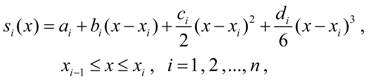
Let continuous function is given on segment [ a , b ]. We’ll enter fragmentation of the segment:

(6)

also we’ll designate , .

Spline corresponding given function and nodes of interpolation (6) is the function , satisfying the following conditions:

1) on each of segments , function is a cubic polynomial;

2) function , and also its the first and the second derivatives are continuous on segment [ a , b ];

3)

The third condition refers to as interpolation condition. The spline defined by conditions 1) – 3), refers to interpolation cubic spline .

Let's consider a way of cubic spline construction [2].

On each of segments , we’ll search for spline-function in the form of the third degree polynomial:

(7)

where found coefficients.

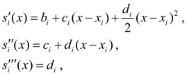
Let’s differentiate (7) three times on х:

hence

From the interpolation condition 3) we recieve:

.       (8)

Besides we’ll consider .

From conditions of function continuity follows:

From here in view of (7) we’ll receive:

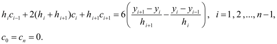
Having designated and lowering intermediate calculations [2], we’ll finally receive the system of equations for definition of coefficients :

(9)

By virtue of matrix of coefficients is three-diagonal the system (9) has the unique solution [2].

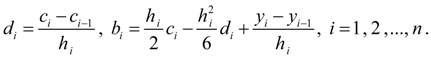
Having found coefficients , other coefficients we’ll define from the open formulas:

(10)

Thus, the unique cubic spline, satisfying to conditions 1) –  3) exists and is found.