Euler's method

Let's consider the differential equation

(1)

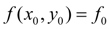
with an initial condition

Substituting into the equation (1), we’ll receive value of a derivative in a point :

At small the following expression takes place:

Designating , let’s rewrite the last equality in the form of:

(2)

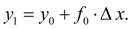
Accepting now for a new initial point, precisely also we’ll receive

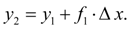
In the general case we’ll have:

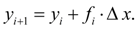(3)

It also is Euler's method . The value refers to as step of integration . Using this method, we receive the approached values у , at as the derivative actually does not remain to a constant on an interval in length . Therefore we receive a mistake in definition of value of function у , that greater, than is more. Euler's method is the elementary method of numerical integration of differential equations and systems. Its defects are a small accuracy and a regular accumulation of mistakes.

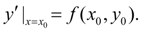
More exact is Euler's modified method with recalculation . Its essence that at the first we find from the formula (3) so-called «a gross approach» (prediction):

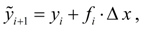
and then the recalculation 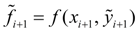gives us too approached, but more exact value (correction):

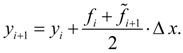(4)

Actually the recalculation allows to consider, though approximately, a change of a derivative on a step of integration as its values in the beginning and in the end of a step (Fig. 1) are considered, and then their average is chosen. Euler's method with recalculation (4) is in essence the 2-nd order Runge-Kutta method [2]. This will become obvious of the further.

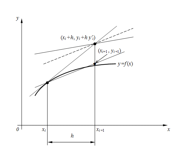
Fig. 1. The geometric representation of Euler’s method with recalculation.