Contents
>> Applied Mathematics
>> Numerical Methods
>> Ordinary Differential Equations
>> Examples
|
Ordinary differential equations - Example
Example
[1].
Calculate by the Runge-Kutta’s method integral of the differential equation
 at the initial condition
 on the segment [0, 0.5] with the step of integration

S o l u t i o n. Let’s calculate
 . For this purpose at the first we’ll consistently calculate
 :
:
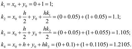
Now we receive:
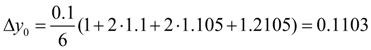
and, consequently,
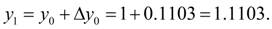
The subsequent approaches are similarly calculated. Results of calculations are tabulated:
Results of numerical integration of the differential
equation (1) by the fourth order Runge-Kutta’s method
|
i
|
x
|
y
|
k
=
0.1
(
x
+
y
)
|
Δ
y
|
|
0
|
1
|
1
|
1
|
0.1
|
|
|
0.05
|
1.05
|
1.1
|
0.22
|
|
|
0.05
|
1.055
|
1.105
|
0.221
|
|
|
0.1
|
1.1105
|
1.210
|
0.1210
|
|
|
|
|
|
1/6
 0.6620=
0.1103
0.6620=
0.1103
|
|
1
|
0.1
|
1.1103
|
1.210
|
0.1210
|
|
|
0.15
|
1.1708
|
1.321
|
0.2642
|
|
|
0.15
|
1.1763
|
1.326
|
0.2652
|
|
|
0.2
|
1.2429
|
1.443
|
0.1443
|
|
|
|
|
|
1/6
0.7947=
0.1324
|
|
2
|
0.2
|
1.2427
|
1.443
|
0.1443
|
|
|
0.25
|
1.3149
|
1.565
|
0.3130
|
|
|
0.25
|
1.3209
|
1.571
|
0.3142
|
|
|
0.3
|
1.3998
|
1.700
|
0.1700
|
|
|
|
|
|
1/6
0.9415=
0.1569
|
|
3
|
0.3
|
1.3996
|
1.700
|
0.1700
|
|
|
0.35
|
1.4846
|
1.835
|
0.3670
|
|
|
0.35
|
1.4904
|
1.840
|
0.3680
|
|
|
0.4
|
1.5836
|
1.984
|
0.1984
|
|
|
|
|
|
1/6
1.1034=
0.1840
|
|
4
|
0.4
|
1.5836
|
1.984
|
0.1984
|
|
|
0.45
|
1.6828
|
2.133
|
0.4266
|
|
|
0.45
|
1.6902
|
2.140
|
0.4280
|
|
|
0.5
|
1.7976
|
2.298
|
0.2298
|
|
|
|
|
|
1/6
1.2828=
0.
2138
|
|
5
|
0.5
|
1.7974
|
|
|
So
,
у
(0.5) =1.7974.
For comparison the exact decision of the differential equation (1) is:
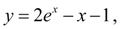
whence
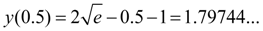
Thus, exact and numerical solutions of the equation (1) have coincided up to the fourth decimal place.
The fourth order Runge-Kutta’s method also is widely applied to the numerical solution of systems of ordinary differential equations.
|