Method of solution

To solve of system of the nonlinear equations (1) we’ll apply the iterative Newton-Raphson method which general scheme is reduced to the following.

Let the system of nonlinear equations is given:

(2)

where x ₁ ,…, x _N – unknowns entering into the equations, F _i – nonlinear functions.

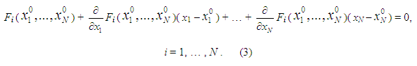
Decomposing F _i ( x ₁ ,…, x _N ) in a power series in a neighborhood of zero approach and keeping only linear members of decomposition, we’ll receive:

The system of the linearized equations (3) in the matrix form can be led to a kind:

(4)

where A [ x ⁰ ], B [ x ⁰ ] – accordingly a matrix of coefficients F _i (Jacoby’s matrix) and a column of right parts of equations, depending on zero approach x ⁰ ; x – a vector of unknowns: ( x ₁ ,…, x _N ). On the n -th iteration the system of equations (4) becomes:

(5)

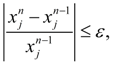
where x ^{n -1} – the solution received on previous ( n – 1)-th iteration.

Thus, on n -th iteration on values x ^{n -1} matrixes A [ x ^{n -1} ] and B [ x ^{n -1} ] are calculated, and then the system of linear equations (5) is solved, therefore x ⁿ is defined.

The process repeats until the given accuracy ε will be satisfied on everyone j -th a component of the vector x ⁿ :

j = 1, … , N .      (6)

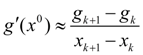
Convergence of the iterative Newton-Raphson process appreciably depends on a choice of zero approach.

Thus, Newton-Raphson algorithm is reduced to consecutive performance of following stages of the problem solution:

1) linearization (3) of initial equations in a neighborhood of the previous iteration (zero approach);

2) giving of input data and zero approach;

3) forming for each iteration of Jacoby’s matrix and a column of right parts for system of linearizated equations (5);

4) solving on each iteration of the generated system of linear equations (5), for example, by Gauss’s method;

5) comparison of two neighboring iterations by a condition of convergence (6) with the given accuracy.

Linearization of the nonlinear equations is a necessary preparatory stage as a result of which the algorithm and the program of the solution of the traction calculation problem are under construction. For realization of iterative process all graphic characteristics M ( ω _e ), ρλ _1,2 ( i ), δ =f ( R ) are approximated by finite sets of points: g ( x ) ~ ( g _k , x _k ), k = 1, …, 10, and the first derivatives of functions ρλ _1,2 ( i ) и δ =f ( R ), appearing owing to linearization of the equations in a point х ⁰ (or x ^{n -1} ) are replaced by their finite-difference relations:

,    and besides x _k ≤ х ⁰ ≤ x _{k +1} . (7)

Input data and zero approach are given by the user directly ahead of start of the computing program. Other points 3) – 5) are realized automatically during the program executing.

If the condition (6) is satisfied, an iterative cycle for given value Т comes to an end, the following parameters are calculated: the engine and the hydraulic torque converter power and efficiency, traction power, the hour charge of fuel and some other, value Т increases for value of the given step ΔТ and unknowns on a new iterative cycle are defined. As a result the traction characteristic corresponding all range of change of traction force T . If a condition (6) is not satisfied, the iterative cycle for given value Т either proceeds before its performance, or interrupts at too big number of executed iterations (from above 20). In this case the corresponding message stands out and it is necessary for user to check up and probably to correct some parameters of calculation (to change zero approach, the step ΔТ , to increase the admission ε, etc.).