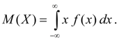
Numerical characteristics of random variables

Mathematical expectation. Mathematical expectation of discrete random variable X accepting finite number of values х _i with probabilities р _i , is the sum:

М ( Х ) = х ₁ · р ₁ + х ₂ · р ₂ + х ₃ · р ₃ + ... + х _n · р _n . (6 а )

Mathematical expectation of continuous random variable X is the integral from product of its values х and its density function f ( x ):

(6 b )

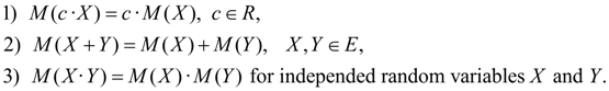
Not own integral (6 b ) is supposed absolutely converging (otherwise, mathematical expectation M ( X ) does not exist).

Mathematical expectation characterizes average value of random variable X . Its dimension coincides with dimension of random variable.

Properties of mathematical expectation:

(7)

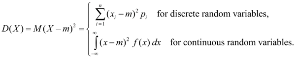
Dispersion. Dispersion of random variable X is the number:

(8)

The dispersion is characteristic of dissipation of random variable X values relatively its average value of M ( X ). Dimension of dispersion is equal to dimension of random variable square. Proceeding from definitions of dispersion (8) and mathematical expectation (5) for discrete random variable and (6) for continuous random variable we’ll receive similar expressions for dispersion:

(9)

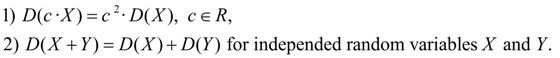
Here m = М ( Х ).

Properties of dispersion:

(10)

Average square-law deviation:

(11)

As dimension of average square-law deviation the same, as at random variable, it is used as measure of dissipation more often, than dispersion.

Moments of distribution. Concepts of mathematical expectation and dispersion are special cases of more general concept for numerical characteristics of random variables – moments of distribution . Moments of distribution of random variable are entered as mathematical expectations of some elementary functions of random variable. So, the k ordermoment relatively point х ₀ is called mathematical expectation M ( X – х ₀ ) ^k . Moments relatively beginning of coordinates х = 0 are called initial moments and are designated:

(12)

Initial moment of the first order is centre value of distribution of considered random variable:

(13)

Moments relatively centre value of distribution х = m are called central moments and are designated:

(14)

From (7) follows, that central moment of the first order is always equal to zero:

(15)

Central moments do not depend on reference mark of random variable values as at shift on constant value C its centre value of distribution moves on the same value C , and deviation from the center does not vary: Х – m = ( Х – С ) – ( m – С ).

Now it is obvious, that dispersion is central moment of the second order :

(16)

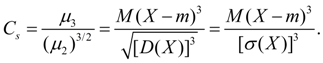
Asymmetry. Central moment of the third order:

(17)

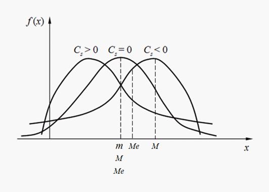
serves for estimation of asymmetry of distribution . If distribution is symmetric relatively point х = m then central moment of the third order will be equal to zero (as well as all central moments of odd orders). Therefore, if central moment of the third order is distinct from zero distribution cannot be symmetric. Value of asymmetry estimate by means of dimensionless coefficient of asymmetry :

(18)

The sign of coefficient of asymmetry (18) specifies right-hand or left-hand sided asymmetry (Fig. 2).

Fig. 2. Kinds of asymmetry of distributions.

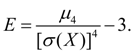
Excess. Central moment of the fourth order:

(19)

serves for estimation of so-called excess defining degree of slope (acute vertex) of curve of distribution near to centre value of distribution in relation to normal distribution curve. As for normal distribution as an excess the value is accepted:

(20)

On Fig. 3 examples of curves of distribution with various values of excess are shown. For normal distribution Е = 0. Curves with more acute vertices, than normal one, have a positive excess, with more plane vertices – negative excess.

Fig. 3. Curves of distributions with various degree of slope (excess).

Moments of higher orders in engineering applications of mathematical statistics usually are not applied.

Mode of discrete random variable is its most probable value. Mode of c ontinuous random variable is its value at which density function is maximal (Fig. 2). If curve of distribution has one maximum, then its distribution refers to unimodal . If curve of distribution has more than one maximum, then its distribution refers to polymodal . Sometimes there are distributions, which curves have not maximum, but minimum. Such distributions refer to antimodal . Generally mode and mathematical expectation of random variable do not coincide. In that specific case, for modal , i.e. having mode, symmetric distribution and provided that there is mathematical expectation , it coincides with mode and center of distribution symmetry.

Median of random variable X is its value Ме for which the equality: takes place, i.e. equiprobably, that random variable X is less or more Ме . Vectorially median is abscissa of point in which area under curve of distribution halves (Fig. 2). In case of symmetric modal distribution median, mode and mathematical expectation coincide.