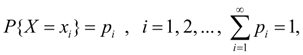
Random variables and distribution laws

Variable is called random if as result of experience it can accept valid values with certain probabilities. The fullest, exhaustive characteristic of random variable is law of distribution . Law of distribution  is function (given by table, graph or formula), allowing to define probability of that random variable X accepts certain value х _i or gets in some interval. If random variable has given law of distribution speak, that it is distributed under this law or submits to this law of distribution.

Random variable X is called discrete if there is such non-negative function

(1)

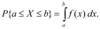
which puts in conformity to value х _i of variable X probability р _i with which it accepts this value.

Random variable X is called continuous if for any a < b there is such non-negative function f ( x ), that

(2)

Function f ( x ) is called density function of continuous random variable.

Probability of that random variable X (discrete or continuous) accepts value, smaller х , is called distribution function of random variable X and is designated F ( x ):

(3)

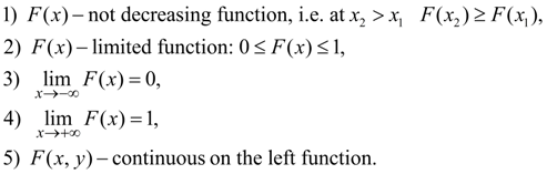
Distribution function is universal kind of distribution law, suitable for any random variable.

Basic properties of distribution function:

(4)

Except for this universal, there are also private kinds of distribution laws: series of distribution (only for discrete random variables) and density function (only for continuous random variables).

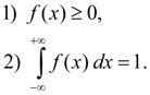
Basic properties of density function:

(5)

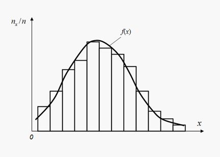
Each law of distribution is some function completely describing random variable according to probable point of view. In practice often it is necessary to discuss about distribution of probabilities of random variable X only by results of tests. Repeating tests, each time let’s register, whether there was interesting us random event A or not. Relative frequency (or simply frequency ) of random event A is called relation of number n _A of occurrences of this event to general number n of executed tests. Thus we accept that relative frequencies of random events are close to their probabilities. It is especially true, than it is more number of executed experiences. Thus of frequencies, as well as probabilities, it is necessary to carry not to separate values of random variable, but to intervals. It means that all range of possible values of random variable X should be broken into intervals. Spending series of tests, giving empirical values of variable X , it is necessary to fix numbers n _x of hits of results in each interval. At the big number of tests n the relation n _x / n (frequencies of hit in intervals) should be close to probabilities of hit in these intervals. Dependence of frequencies n _x / n from intervals defines empirical distribution of probabilities of random variable X which graphic representation refers to as histogram (Fig. 1).

Fig. 1. Histogram and aligning density function

For construction of histogram on x -axis intervals of equal length are set into which all range of possible values of random variable X is broken, and on y -axis frequencies n _x / n are set. Then height of each column of histogram is equal to corresponding frequency. Thus, the approached representation of law of distribution of probabilities for random variable X in form of step function turns out, approximation (alignment) of which by some curve f ( x ) will give density function.

However, often happens to specify enough only separate numerical parameters describing basic properties of distribution. These numbers are called numerical characteristics of random variable.