Distributions of discrete random variables

Binomial distribution. Discrete random variable X has binomial distribution , if its possible values 0, 1, 2..., m , …, n , and probabilities corresponding them are equal to:

(21)

where 0 < p < 1, q = 1 – p ; m = 0, 1, 2, ... , n .

As shown from (21), probabilities Р _т are calculated, as members of decomposition of Newton’s binomial , whence and the name «binomial distribution».

Example is selective quality assurance of industrial products at which selection of products for test is made on the scheme of casual repeated sample i.e. when the checked up products come back in an initial party. Then the quantity of non-standard products among selected is a random variable with the binomial law of distribution.

Binomial distribution is defined by the two parameters: n and p . Random variable distributed according to binomial law, has the following basic numerical characteristics:

(22)

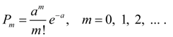
Poisson’s distribution. Discrete random variable X has Poisson’s distribution if it has infinite calculating set of possible values 0, 1, 2..., m , …, and probabilities corresponding them are defined by the formula:

(23)

Examples of the casual phenomena, subordinated to Poisson’s distribution law, are: sequence of radioactive disintegration of particles, sequence of refusals at work of complex computer system, a stream of applications on a telephone exchange and many other things.

Poisson’s distribution law (23) depends on one parameter а which simultaneously is both a mathematical expectation, and a dispersion of random variable X distributed according to Poisson’s law. Thus, for Poisson’s distribution law the following basic numerical characteristics take place:

(24)

Geometrical distribution. Discrete random variable X has geometrical distribution, if its possible values 0, 1, 2..., m , …, and probabilities of these values:

(25)

where 0 < p < 1, q = 1 – p ; m = 0, 1, 2, ... .

Probabilities Р _т for consecutive values m form a geometrical progression with the first member р and denominator q , whence and the name «geometrical distribution».

As an example we’ll consider shooting on some purpose before the first hit , and the probability of hit at each shot does not depend on results of the previous shots and keeps constant value р (0 < p <1). Then the quantity of the made shots will be a random variable with geometrical distribution of probabilities.

Geometrical distribution is defined by one parameter р . Random variable, subordinated to the geometrical law of distribution, has the following basic numerical characteristics:

(26)

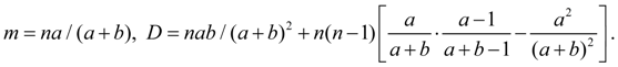
Hyper geometrical distribution. Discrete random variable X has hyper geometrical distribution with parameters a , b , n , if its possible values 0, 1, 2, ... , m , … , a have probabilities:

(27)

Hyper geometrical distribution arises, for example, when from an urn containing a black and b of white spheres, take out n spheres. A random variable, subordinated to the hyper geometrical law of distribution, is the number of white spheres among taken out. The basic numerical characteristics of this random variable:

(28)