Regression analysis. The least squares smoothing

One of often meeting problems at processing results of experiment is selection of the formula for an establishment of functional dependence between experimental data, the so-called regression equation . Before to start selection of the formula, it is expedient to put empirical data on the graph and approximately, by hand to lead through the received points the most plausible curve. Very often the general view of a curve happens is known from other reasons that simplifies a problem, reducing it to search of numerical coefficients of known functional dependence of a general view (for example, linear, square-law, logarithmic, etc.). Thus those empirical data that most likely contain the greatest errors become often visible. Except for the received experimental points the essential moment at carrying out of a curve are reasons of the general character: as the curve near to zero behaves, whether it crosses coordinate axes, whether touch es them, whether has asymptotes, etc.

After this preliminary work is done, selection of the formula – the equations of regress begins actually. In solution of the problems connected with search of the equations of regress is engaged regression analysis , and one of it of algorithms most widely put into practice is the method of the least squares [3, 5, 6, 7].

Generally the method of the least squares problem is formulated as follows. Let required functional dependence of value y from value х is expressed by the formula:

(1)

where given functions, found parameters – coefficients of the equation (1).

It is supposed, that values of argument х are established precisely, and corresponding values of function y are defined in experiment with some error. If measurements were made without mistakes for definition of parameters it would be required exactly т +1 measurements. But because of mistakes of experiment different series from т +1 measurements will give various values of parameters . Therefore the quantity of spent measurements should be much more, than number m of defined parameters, for reduction of influence of mistakes of experiment due to use of a surplus information and receiving of the best somewhat estimations of defined parameters.

So, for receiving of estimations of parameters it is spent n experiments which results give value not these parameters, and some function (1) depending on them linearly.

The method of the least squares consists that estimations of parameters of the formula (1) are defined from a condition: the sum of squares of deviations

(2)

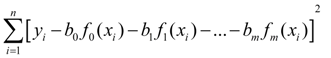
reaches the least value.

It is necessary for definition of these estimations to differentiate (2) by all estimations , to equate all derivatives to zero and to solve the received linear system from т +1 equations rather т +1 unknown estimations of parameters :

(3)

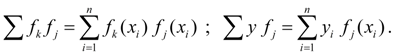
The system of the equations (3) refers to as system of Gauss’ normal equations .

Here for brevity records the following designations of the sums are accepted:

(4)

It is necessary to note, that the system of the equations (3) sometimes appears ill-conditioned , i.e. its solutions are rather sensitive to the slightest changes in results of measurements. Special methods now are developed for ill-conditioned systems, for example, regularization methods.