Method of finite differences (method of grids)

Idea of a method of finite differences (method of grids) is known for a long time, from Euler's corresponding works. However practical application of this method was then is rather limited because of huge volume of manual calculations connected with dimension of received at it systems of algebraic equations on which solution years were required. Now, with the advent of high-speed computers, the situation has radically changed. This method became convenient for practical use and is one of the most effective at the solution of various problems of mathematical physics.

Basic idea of method of finite differences (method of grids) for the approached numerical solution of boundary value problem for bidimentional partial differential equation consists in that

1) on a plane in field A in which the solution is searched, grid area А _s (Fig.1), consisting of identical cells in size s ( s – step of grid) and being approach of the given area A is under construction;

2) given partial differential equation is replaced in nodes of grid А _s with the corresponding finite-difference equation;

3) in view of boundary conditions values of the required solution in boundary nodes of area А _s are established.

Fig. 1. Construction of grid area

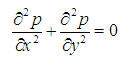
Solving the received system of finite-difference algebraic equations, we’ll receive values of required function in nodes of grid А _s , i.e. the approached numerical solution of boundary value problem.

The choice of grid area А _s depends on specific problem, but always it is necessary to aspire to that a contour of grid area А _s in the best way approximated a contour of area A .

Let's consider Laplace’s equation

,       (1)

where p ( x , y ) – required function, x , y – rectangular coordinates of flat area and let’s receive the corresponding it finite-difference equation.

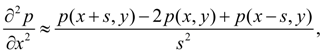
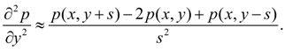
Let's replace private derivatives and in the equation (1) with finite-difference relations:

Then solving the equation (1) in p ( x , y ), we shall receive:

p ( x , y ) = [ p ( x + s , y ) + p ( x – s , y ) + p ( x , y + s ) + p ( x , y – s ) ] / 4.         (2)

Having set values of function p ( x , y ) in boundary nodes of a contour of grid area А _s according to boundary conditions and solving the received system of equations (2) for each node of grid, we’ll receive the numerical decision of the boundary value problem (1) in the given area A .

Clearly, that number of equations of a kind (2) is equal to quantity of nodes of grid area А _s , and than it is more nodes (i.e. the more finely grid), then error of calculations is less. However it is necessary to remember, that with reduction of a step s dimension of system of equations and therefore, solving time increases. Therefore all over again it is recommended to execute trial calculations with enough big step s , to estimate the received error of calculations, and only then to pass to finer grid in all area or in its any part.