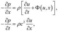
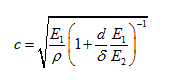
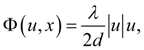
Method of characteristics

Method of characteristics is a method of numerical integration of systems of partial differential equations of hyperbolic type. For the first time for some special cases it has been considered in D’Alembert’s proceedings. Now the method of characteristics is widely applied in problems of distribution of waves in hydro- air- dynamics. So, dynamics of liquid flow in view of distributed parameters on length of pipeline (pressure, flow speed, mass, viscous friction) is described by the system of quasi-linear hyperbolic partial differential equations [4–6]:

(18)

where p, u – average on section pressure and speed of liquid flow; t – time; х – coordinate on pipe length; ρ – liquid density; – the sound speed in a liquid in view of elasticity of pipeline walls; Е ₁ – the volumetric module of elasticity of a liquid; Е ₂ – the module of elasticity of a material of a pipe; d , δ – internal diameter and thickness of a wall of the pipeline; Φ ( u , x ) – nonlinear function of viscous friction. For the pipeline of round section where λ – coefficient of hydraulic resistance depending on Reynolds’ number Re = u d / ν , here ν – kinematic viscosity of a liquid.

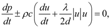
Integration of the nonlinear equations (18) we’ll execute by numerical method of characteristics according to which the initial partial differential equations (18) are replaced with the ordinary differential equations

(19)

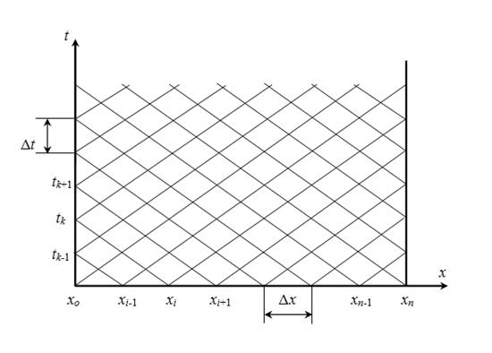
taking place along direct and return characteristics dx = ± c dt.

Numerical integration of the equations (19) by method of characteristics is carried out as follows. On plane xt (Fig.4) a grid of direct and return characteristics is under construction, and a step of integration on length Δ x is connected with step of integration on time Δ t by linear correlation: Δ x = c Δ t . After transition in the equations (19) to finite differences in view of given boundary conditions we solve the received system of equations by method of iterations.

Fig.4. Construction of direct and return characteristics

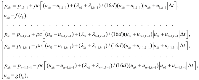
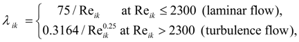
Let's consider the problem (18) – (19) solution by method of characteristics at the certain boundary conditions. We’ll enter in nodes of grid of characteristics (Fig.4) the following designations: p ( x _i , t _k ) = p _ik ; u ( x _i , t _k ) = u _ik ; λ ( x _i , t _k ) = λ _ik . Then in view of boundary conditions u _ok = f ( t _k ), u _nk = g ( t _k ) after exchanging in equations (19) derivatives by finite-difference relations, and variables p, u and λ – their average values in the neighbor nodes of grid on direct and return characteristics [accordingly ( x _i , t _k ), ( x _{i -1} , t _{k -1} ) and ( x _i , t _k ), ( x _{i +1} , t _{k -1} )], we’ll receive the following system of nonlinear algebraic equations:

(20)

(21)

where .

The received system of equations (20) – (21) is solved by an iterative method.